Exploring Dominant Spatial Patterns with a Single Variable
In this post, we delve into the formal exploration of dominant spatial patterns, particularly in the context of climate research.
Understanding Spatial Patterns
In climate research, the interpretation of physical phenomena and spatial variations often involves the application of dominant spatial patterns. For instance, consider the two major spatial patterns (modes) of sea surface temperature in the Indian Ocean: the basin mode and the dipole mode.
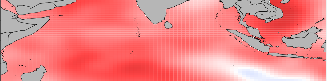


These patterns play a crucial role in deciphering the spatial variation of climate variables, such as sea surface temperature, with implications for phenomena like El Niño–Southern Oscillation (ENSO).
Mathematical Formalization of Spatial Patterns
Spatial Process of Interest
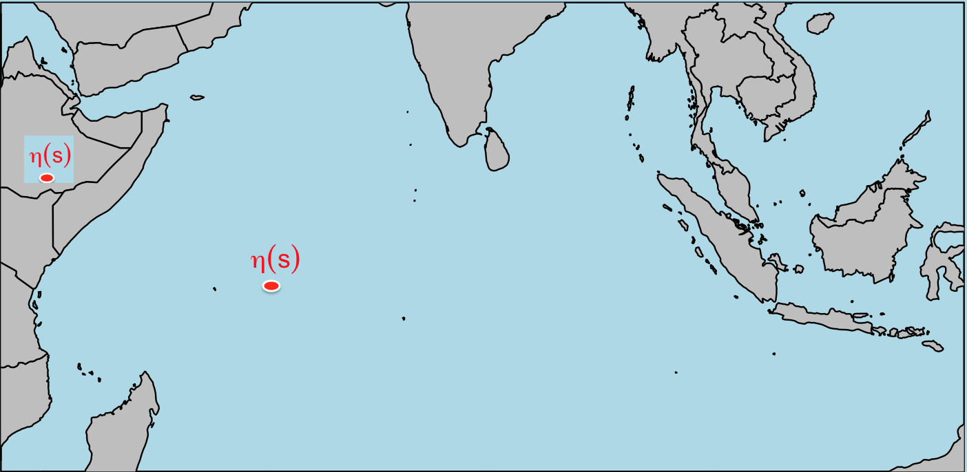
Let’s consider a spatial process denoted as \(\{\eta_i(\cdot); i = 1,\dots, n\}\) representing a climate variable over a region $D \subset \mathbb{R}^d$ at $n$ different time points. The process is assumed to be mean zero, mutually uncorrelated, and characterized by a common covariance function.
For example, we are interested in studying sea surface temperature monthly anomalies in the Indian Ocean during Jan., 2010 to Dec. 2016, formally. Then, we can define $\eta_i(\cdot)$ as a sea surface temperature monthly anomaly, $D$ as Indian Ocean (with blue color in the following plot), $n = 12\times 7$.
Observed Data
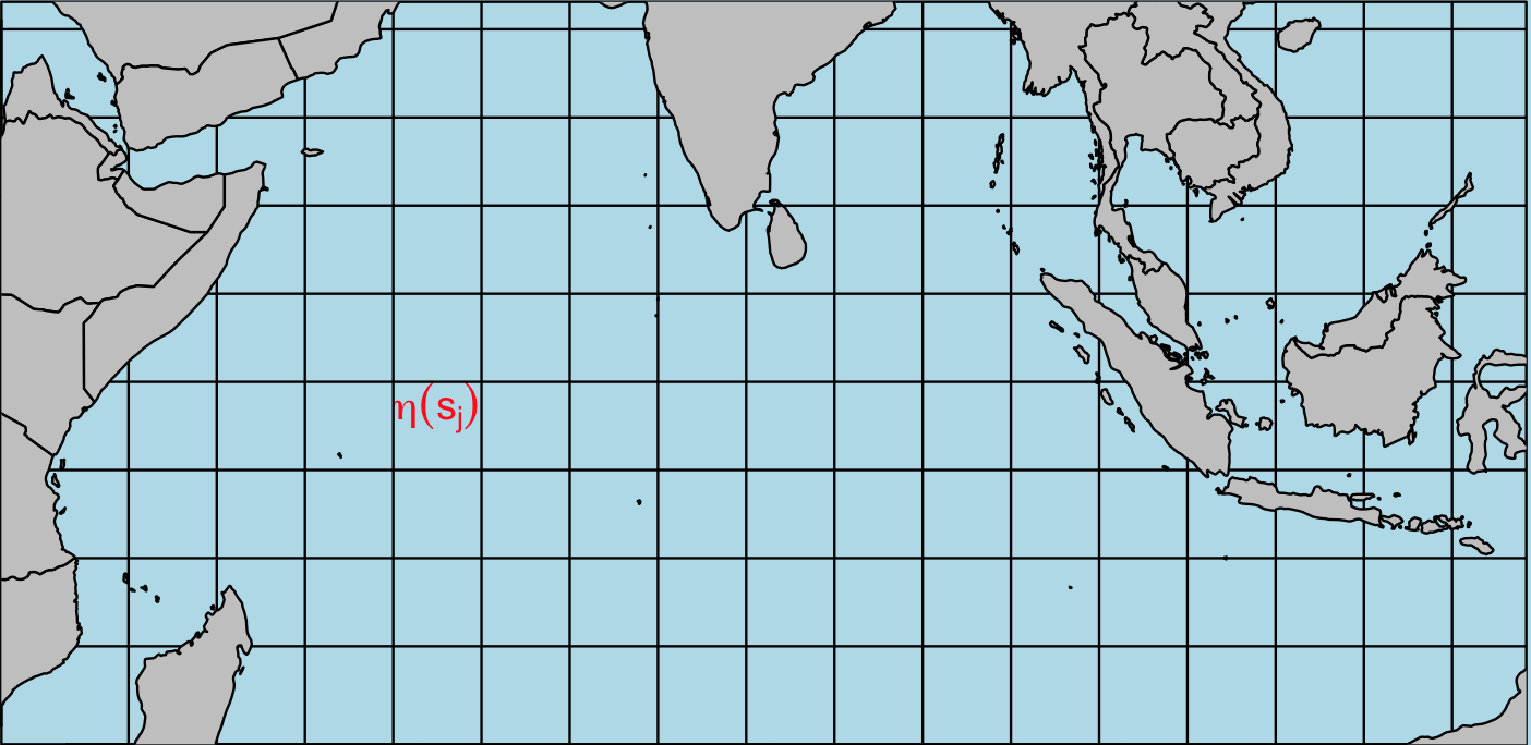
Observations are available at $p$ locations, denoted as $s_1, \dots, s_p$. The observed data at these locations are defined as \(Y_i(s_j) = \eta_i(s_j) + \epsilon_{ij},\) where $\epsilon_{ij}$ represents white noise with mean zero and covariance $\sigma^2$ for $i =1,\dots,n$ and $j = 1, \dots,p$.
The graph below indicates that the observation at some cell, where the size of cells depends on the resolution of measurement. By the way, the gray color represent the land, and the observation here is usually define as $NA$ in datasets.
We can rewrite our data as a matrix form. Namely, $\textbf{Y} = (\textbf{Y}_1, \dots, \textbf{Y}_n)’$ is an $n\times p$ matrix where, at each time point, we vectorize our observations over $p$ locations as $\textbf{Y}_i = (Y_i(s_1), \dots,Y_i(s_p))’$, $i = 1, \dots n$.
Spatial Patterns via Principal Component Analysis (PCA)
Assuming $\textbf{Y}\sim(\textbf{0}, \Sigma)$, Principal Component Analysis (PCA) aims to find directions, $\bf{\phi}\in \mathbb{R}^{p\times 1}$, maximizing the variance of $\textbf{Y}_i$ projected onto $\bf{\phi}$. The first $K$ eigenvectors of the estimated covariance matrix $\textbf{S}$ provide the dominant spatial patterns.
In practice, these patterns, often referred to as empirical orthogonal functions (EOF), are crucial for interpreting spatial variations, especially in irregular-location data.
Summary
The article explores the formalization of dominant spatial patterns, particularly in climate research. It introduces the concept of spatial patterns, essential in interpreting physical phenomena and spatial variations in climate variables. Using examples from sea surface temperature in the Indian Ocean, the article illustrates basin and dipole modes as significant spatial patterns. The mathematical formalization involves defining a spatial process of interest, observing data at specific locations, and employing Principal Component Analysis (PCA) to identify dominant spatial patterns. The insights gained from these patterns contribute to understanding climate variations and phenomena like El Niño–Southern Oscillation.
References
- Wang and Huang (2017). Regularized Principal Component Analysis for Spatial Data.