Apply SpatPCA to Capture the Dominant Spatial Pattern with One-Dimensional Locations
In this tutorial, we explore the application of SpatPCA to capture the most dominant spatial patterns in one-dimensional data, highlighting its performance under varying signal-to-noise ratios.
Basic Settings
Used Packages
library(SpatPCA)
library(ggplot2)
library(dplyr)
library(tidyr)
library(gifski)
base_theme <- theme_classic(base_size = 18, base_family = "Times")
True Spatial Pattern (Eigenfunction)
The underlying spatial pattern exhibits significant variation at the center and remains nearly unchanged at both ends of the curve.
set.seed(1024)
position <- matrix(seq(-5, 5, length = 100))
true_eigen_fn <- exp(-position^2) / norm(exp(-position^2), "F")

data.frame(
  position = position,
  eigenfunction = true_eigen_fn
) %>%
  ggplot(aes(position, eigenfunction)) +
  geom_line() +
  base_theme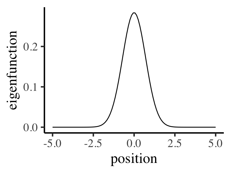
Case I: Higher Signal of the True Eigenfunction
Generate Realizations
We generate 100 random samples based on a spatial signal with a standard deviation of 20 and standard normal distribution for noise.
realizations <- rnorm(n = 100, sd = 20) %*% t(true_eigen_fn) + matrix(rnorm(n = 100 * 100), 100, 100)Animate Realizations
Simulated central realizations exhibit a wider range of variation than others.
for (i in 1:100) {
  plot(x = position, y = realizations[i, ], ylim = c(-10, 10), ylab = "realization")
}
Apply SpatPCA::spatpca
cv <- spatpca(x = position, Y = realizations)
eigen_est <- cv$eigenfn
Compare SpatPCA with PCA
Comparison reveals that SpatPCA provides sparser patterns than PCA, closely resembling the true eigenfunction.
data.frame(
  position = position,
  true = true_eigen_fn,
  spatpca = eigen_est[, 1],
  pca = svd(realizations)$v[, 1]
) %>%
  gather(estimate, eigenfunction, -position) %>%
  ggplot(aes(x = position, y = eigenfunction, color = estimate)) +
  geom_line() +
  base_theme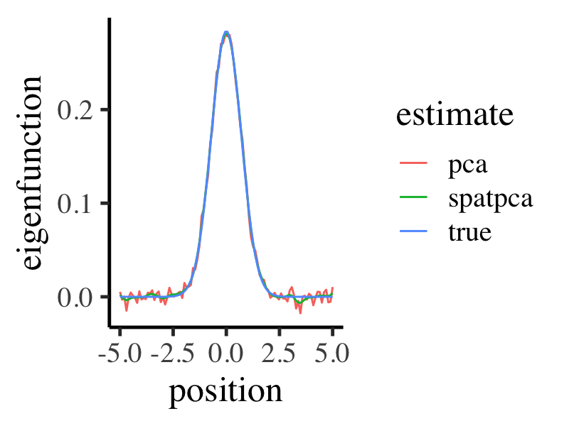
Case II: Lower Signal of the True Eigenfunction
Generate Realizations with $\sigma=3$
realizations <- rnorm(n = 100, sd = 3) %*% t(true_eigen_fn) + matrix(rnorm(n = 100 * 100), 100, 100)Animate Realizations
Simulated samples show a less clear spatial pattern.
for (i in 1:100) {
  plot(x = position, y = realizations[i, ], ylim = c(-10, 10), ylab = "realization")
}
Compare Resultant Patterns
SpatPCA outperforms PCA visually when the signal-to-noise ratio is lower.
cv <- spatpca(x = position, Y = realizations)
eigen_est <- cv$eigenfn

data.frame(
  position = position,
  true = true_eigen_fn,
  spatpca = eigen_est[, 1],
  pca = svd(realizations)$v[, 1]
) %>%
  gather(estimate, eigenfunction, -position) %>%
  ggplot(aes(x = position, y = eigenfunction, color = estimate)) +
  geom_line() +
  base_theme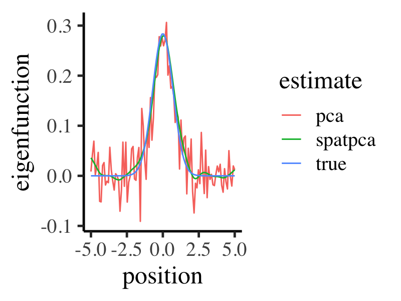
Summary
In this article, we explore the application of the SpatPCA R package to capture dominant spatial patterns in one-dimensional data. The tutorial focuses on demonstrating SpatPCA’s performance under different signal-to-noise ratios. Two cases are considered: one with a higher signal and another with a lower signal. Animated realizations and comparisons with traditional PCA illustrate SpatPCA’s ability to provide sparser and more accurate patterns, particularly in scenarios with lower signal-to-noise ratios.