Capturing Dominant Spatial Patterns with Two-Dimensional Locations Using SpatPCA

In this demonstration, we showcase how to utilize SpatPCA for analyzing two-dimensional data to capture the most dominant spatial pattern.

Basic Settings

Used Packages

library(SpatPCA)
library(ggplot2)
library(dplyr)
library(tidyr)
library(gifski)
library(fields)
library(scico)

base_theme <- theme_minimal(base_size = 10, base_family = "Times") +
  theme(legend.position = "bottom")
fill_bar <- guides(fill = guide_colourbar(
  barwidth = 10,
  barheight = 0.5,
  label.position = "bottom"
))
coltab <- scico(128, palette = "vik")
color_scale_limit <- c(-.28, .28)

True Spatial Pattern (Eigenfunction)

The underlying spatial pattern indicates variations at the center and stability at both ends of the curve.

set.seed(1024)
p <- 30
n <- 50
location <-
  matrix(rep(seq(-5, 5, length = p), 2), nrow = p, ncol = 2)
expanded_location <- expand.grid(location[, 1], location[, 2])
unnormalized_eigen_fn <-
  as.vector(exp(-location[, 1]^2) %*% t(exp(-location[, 2]^2)))
true_eigen_fn <-
  unnormalized_eigen_fn / norm(t(unnormalized_eigen_fn), "F")

data.frame(
  location_dim1 = expanded_location[, 1],
  location_dim2 = expanded_location[, 2],
  eigenfunction = true_eigen_fn
) %>%
  ggplot(aes(location_dim1, location_dim2)) +
  geom_tile(aes(fill = eigenfunction)) +
  scale_fill_gradientn(colours = coltab, limits = color_scale_limit) +
  base_theme +
  labs(title = "True Eigenfunction", fill = "") +
  fill_bar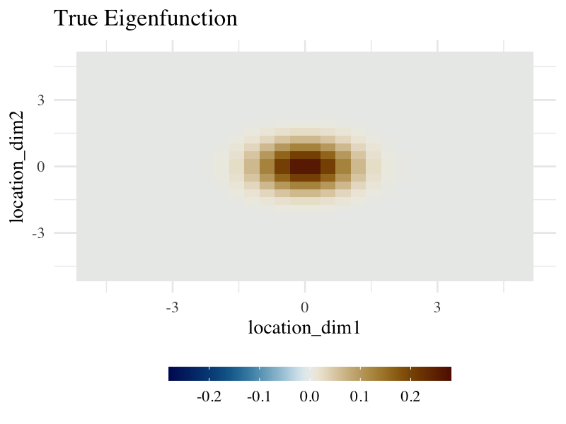

Experiment

Generate 2-D Realizations

Generate 100 random samples based on a spatial signal with $\sigma=20$ and standard normal distribution noise.

realizations <- rnorm(n = n, sd = 10) %*% t(true_eigen_fn) + matrix(rnorm(n = n * p^2), n, p^2)

Animate Realizations

Observe central realizations changing more frequently than others.

for (i in 1:n) {
  par(mar = c(3, 3, 1, 1), family = "Times")
  image.plot(
    matrix(realizations[i, ], p, p),
    main = paste0(i, "-th realization"),
    zlim = c(-10, 10),
    col = coltab,
    horizontal = TRUE,
    cex.main = 0.8,
    cex.axis = 0.5,
    axis.args = list(cex.axis = 0.5),
    legend.width = 0.5
  )
}

Apply `SpatPCA::spatpca`

Add a candidate set of tau2 to observe how SpatPCA obtains a localized smooth pattern.

tau2 <- c(0, exp(seq(log(10), log(400), length = 10)))
cv <- spatpca(x = expanded_location, Y = realizations, tau2 = tau2)
eigen_est <- cv$eigenfn

Compare SpatPCA with PCA

The figure below illustrates that SpatPCA can find a sparser pattern than PCA, which closely matches the true pattern.

data.frame(
  location_dim1 = expanded_location[, 1],
  location_dim2 = expanded_location[, 2],
  spatpca = eigen_est[, 1],
  pca = svd(realizations)$v[, 1]
) %>%
  gather(estimate, eigenfunction, -c(location_dim1, location_dim2)) %>%
  ggplot(aes(location_dim1, location_dim2)) +
  geom_tile(aes(fill = eigenfunction)) +
  scale_fill_gradientn(colours = coltab, limits = color_scale_limit) +
  base_theme +
  facet_wrap(. ~ estimate) +
  labs(fill = "") +
  fill_bar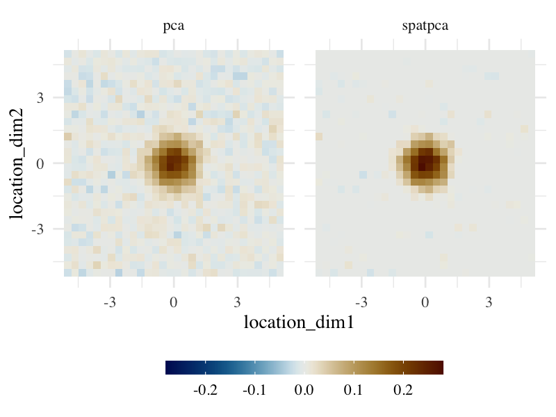

Summary

In conclusion, this tutorial delves into the powerful capabilities of SpatPCA for analyzing spatial patterns in two-dimensional data. By leveraging SpatPCA, we’ve demonstrated its efficacy in capturing dominant spatial patterns through simulated realizations and comparisons with traditional PCA. The intuitive visualizations showcase SpatPCA’s ability to provide localized and smooth eigenfunctions, making it a valuable tool for understanding complex spatial structures.