From PCA to Barlow Twins: A Statistical View of Redundancy Reduction in Self-Supervised Learning

I originally found Barlow Twins confusing for a simple reason: it looks statistical on paper, but it doesn’t behave like PCA when you actually run it.

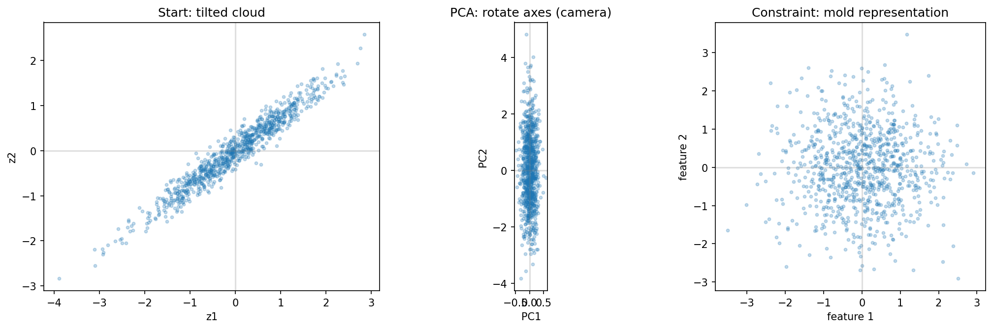
Both methods touch second‑order structure, but they use it at different times and for different purposes. Think of PCA as rotating the camera to fit the data: it takes a cloud of points and rotates the axes until they align with the cloud’s width. Think of Barlow Twins as molding the clay to fit the camera frame: it takes a flexible cloud and squeezes and pulls the cloud itself until it aligns with the axes.

The Problem of Redundancy in Representations

Autoencoders measure success by reconstruction error, but reconstruction quality does not imply statistical efficiency. An autoencoder may perfectly reconstruct images while learning representations with highly correlated dimensions.

Reconstruction alone does not specify how information should be organized across dimensions.

Principal Component Analysis as a Statistical Baseline

PCA operates on the sample covariance matrix:

\[{\mathbf{\hat C}} = \frac{1}{n-1} \sum_{i=1}^n (\mathbf{z}_i - \bar{\mathbf{z}})(\mathbf{z}_i - \bar{\mathbf{z}})^T\]

PCA is a post-hoc transformation: given a fixed representation, it finds an orthogonal basis that diagonalizes the sample covariance.

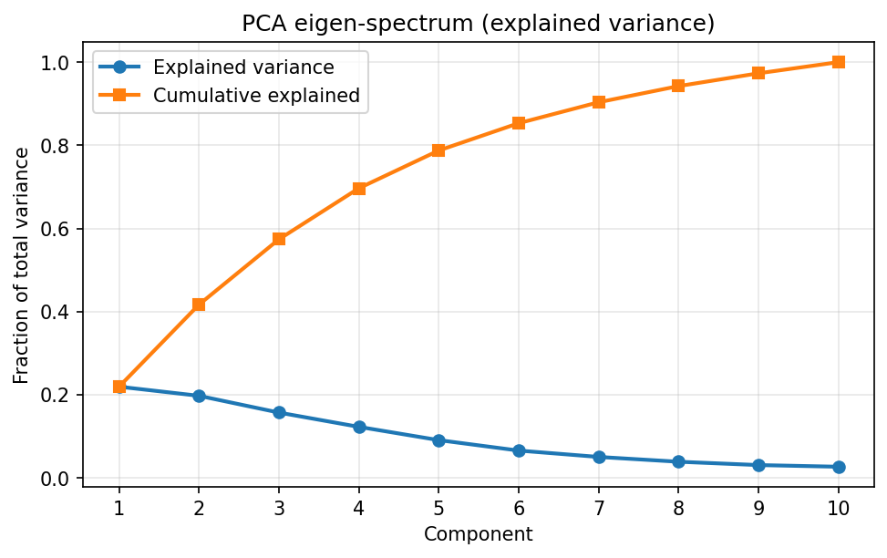
The eigenvectors of ${\mathbf{\hat C}}$ define directions of decreasing variance. In this simulation the spectrum is visibly skewed: most variance lives in a small number of directions, even though the representation is nominally $d$‑dimensional.

PCA eigen-spectrum showing variance explained by each principal component

Figure 1. PCA eigen-spectrum: variance explained by each principal component for the redundant representation.

Barlow Twins: A Statistical Formulation

Barlow Twins is a self-supervised learning method that constrains second-order statistics of learned representations during training.

For each image $\mathbf{x}_i$, we generate two augmented views, $\mathbf{x}_i^A$ and $\mathbf{x}_i^B$, and pass them through a shared network $f_\theta$:

\[\mathbf{z}_i^A = f_\theta(\mathbf{x}_i^A), \quad \mathbf{z}_i^B = f_\theta(\mathbf{x}_i^B)\]

Barlow Twins computes the sample cross-correlation matrix:

\[\mathbf{C}_{ij} = \frac{\sum_{b=1}^B z^A_{b,i} z^B_{b,j}}{\sqrt{\sum_{b=1}^B (z^A_{b,i})^2} \sqrt{\sum_{b=1}^B (z^B_{b,j})^2}}\]

The Barlow Twins objective has two components:

Invariance term: Encourages diagonal elements $C_{ii}$ to be close to 1, making corresponding dimensions from the two views highly correlated (invariance to augmentations).
Redundancy reduction term: Encourages off-diagonal elements $C_{ij}$ (where $i \neq j$) to be close to 0, decorrelating different dimensions.

\[L = \sum_i (1 - C_{ii})^2 + \lambda \sum_i \sum_{j \neq i} C_{ij}^2\]

This objective was introduced by Zbontar et al. (ICML 2021) as a direct implementation of Barlow’s redundancy-reduction principle. The key idea is to make representations invariant across augmentations while explicitly penalizing statistical dependence between feature dimensions without relying on architectural asymmetries such as predictor networks, stop‑gradient tricks, or momentum encoders.

The diagonal term enforces invariance across views, while the off-diagonal penalty discourages duplicated features.

Unlike PCA, this constraint is applied during training. PCA takes a fixed cloud and rotates the coordinate system; Barlow Twins changes the mapping that produces the cloud.

One subtlety that matters for the rest of this post: PCA’s “rotation” is explicit and identifiable (it’s the eigenvector matrix of (\hat{\mathbf{C}})). Barlow Twins does not output a unique rotation you can point to. Once a representation is (approximately) decorrelated, any additional orthogonal rotation preserves that property, so the basis is fundamentally non‑identifiable. In other words: PCA rotates after the fact; Barlow Twins makes redundancy expensive during learning.

Conceptual diagram: PCA rotates axes vs Barlow Twins molds representation

Conceptual view: PCA rotates the coordinate axes to fit the data; Barlow Twins molds the representation to fit the axes.

Schematic of Barlow Twins: two views through a shared network, cross-correlation, and an identity target

Schematic. Two augmented views go through a shared network; training pushes the cross-correlation $\mathbf{C}$ toward the identity.

The toy setup (so the plots have a home)

Before talking about $\lambda$, it helps to say what we’re actually optimizing in this post.

All the figures below use the same small synthetic setup:

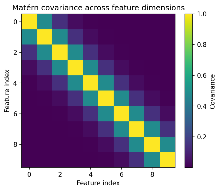
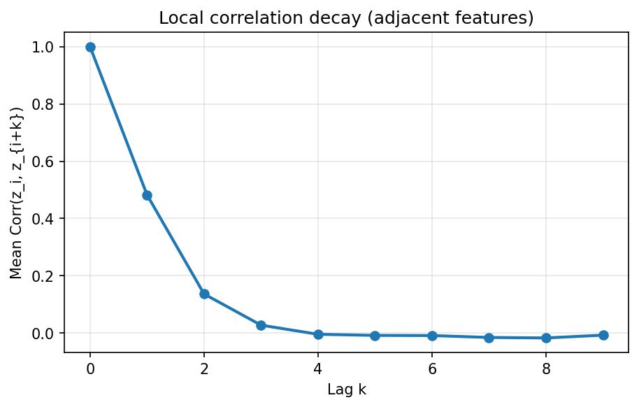
We construct a $d$‑dimensional “redundant” representation $\mathbf{z}$ whose feature–feature covariance is Matérn‑structured (nearby dimensions are strongly correlated; correlation decays with distance).
We create two noisy “views” of the same underlying sample by perturbing $\mathbf{z}$ (think: two augmentations that preserve some signal but add nuisance variation).
Then we learn a linear map $W$ (a stand‑in for a deep encoder) by minimizing the Barlow Twins loss on $(W\mathbf{z}^A, W\mathbf{z}^B)$.

So when you see a $\lambda$ sweep, it’s not abstract hyperparameter tuning: it’s literally showing how the same data and objective shift as we change the price on off‑diagonal correlations.

Why two views, off-diagonals, and λ

Two views provide a nontrivial alignment target: each feature must be predictive across augmentations. Without the off-diagonal penalty, this objective can be satisfied by copying the same signal across many dimensions. The parameter $\lambda$ controls how expensive such duplication is. In the toy setup above, the two “views” are just noisy perturbations of the same latent sample, which is enough to make the alignment constraint non‑trivial.

I find it helpful to think of $\lambda$ as a price on feature duplication: if copying the same signal into many coordinates is cheap, the model will do it.

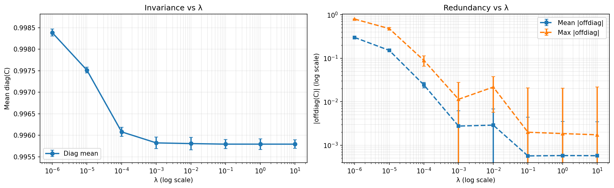
Lambda exploration: invariance vs λ (left) and redundancy vs λ (right) on log scales

Figure 4. Lambda exploration showing the trade-off between invariance (diagonal mean, left) and redundancy reduction (mean and max $\lvert C_{ij}\rvert$ for $i\neq j$, right). Log-scale x-axis spans $\lambda$ from $10^{-6}$ to $10$. Error bars show bootstrap variability from finite-sample estimates.

For small $\lambda$, invariance is already high, but redundancy remains large. Increasing $\lambda$ rapidly suppresses off-diagonal correlations. Beyond $\lambda \approx 10^{-2}$, redundancy approaches a numerical floor in this toy setup, and further increases offer limited additional benefit.

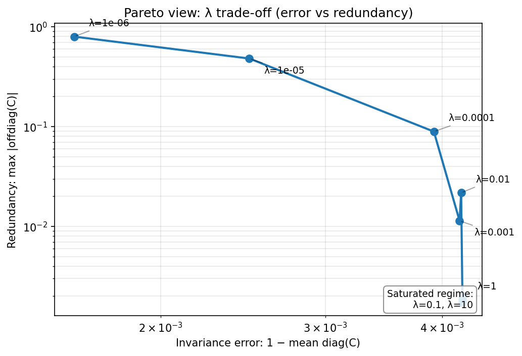
I found Figure 4b helpful because it collapses this trade-off into a single view: moving along the curve corresponds to increasing $\lambda$, with the saturated regime clustering near the bottom-left.

Pareto view of lambda trade-off: invariance error vs redundancy on log-log scale

Figure 4b. Pareto view of the $\lambda$ trade-off: invariance error (1 − mean diag$(\mathbf{C})$) vs redundancy (max $\lvert\mathrm{offdiag}(\mathbf{C})\rvert$) on log-log scale. Moving along the curve corresponds to increasing $\lambda$. The saturated regime ($\lambda \ge 10^{-2}$) clusters near the bottom-left (the "Pareto front"), where you cannot reduce redundancy further without hurting invariance.

Representation efficiency: an information-geometric view

At this point, it’s natural to ask what “less redundancy” actually buys us. Suppressing off-diagonal correlations clearly makes features less duplicated, but is there a more principled way to quantify how efficient a representation really is?

A recent paper by Di Zhang (2025) offers a helpful lens by framing representation learning through information geometry. The key idea is to treat the encoder as inducing a statistical manifold: nearby points in representation space correspond to nearby distributions. The local geometry of this manifold is captured by the Fisher Information Matrix (FIM).

If the FIM spectrum is highly anisotropic, only a few large eigenvalues, then most directions in representation space are effectively wasted. If the spectrum is flat, all directions contribute comparably. Zhang formalizes this intuition by defining representation efficiency [ \eta = \frac{\text{effective intrinsic dimension}}{\text{ambient dimension}}, ] where the effective dimension is derived from the spectral properties of the (average) FIM.

Under simplifying but transparent assumptions: Gaussian representations and augmentations that behave like isotropic noise, the paper shows that driving the Barlow Twins cross-correlation matrix toward the identity induces an isotropic FIM, achieving optimal efficiency ((\eta = 1)). From this perspective, the identity target in Barlow Twins is not arbitrary: it is precisely the condition that equalizes information across dimensions.

This interpretation aligns closely with the empirical behavior we saw above. Increasing (\lambda) flattens the spectrum and removes dominant directions. The information-geometric result explains why this matters: flattening second-order structure increases the number of directions that actually carry information.

Crucially, this does not make Barlow Twins a likelihood-based or generative method. The argument is geometric rather than probabilistic, it concerns how information is distributed across coordinates, not how well a particular density model fits the data. But it clarifies the role of the loss: Barlow Twins is not merely decorrelating features; it is shaping the information geometry of the representation space.

What redundancy looks like (the Matérn toy)

Because the toy covariance is Matérn‑structured, the “raw” representation has a banded correlation pattern: nearby dimensions are redundant and far‑apart ones are less so. This choice matters because real neural network features often exhibit local correlations, filters responding to similar textures, adjacent spatial locations, or semantically related patterns. The Matérn kernel simulates this “smoothness” in feature space, unlike a random Gaussian matrix where dimension 1 and dimension 2 are totally unrelated. This makes the toy example more representative of the structured redundancy that appears in practice.

Matérn covariance heatmap showing smooth correlation across feature dimensions

Matérn covariance structure: correlation decays smoothly with distance between feature indices.

Correlation decay curve showing how correlation decreases with feature distance

Local correlation decay: nearby features (small lag $k$) are highly correlated; distant features are nearly independent.

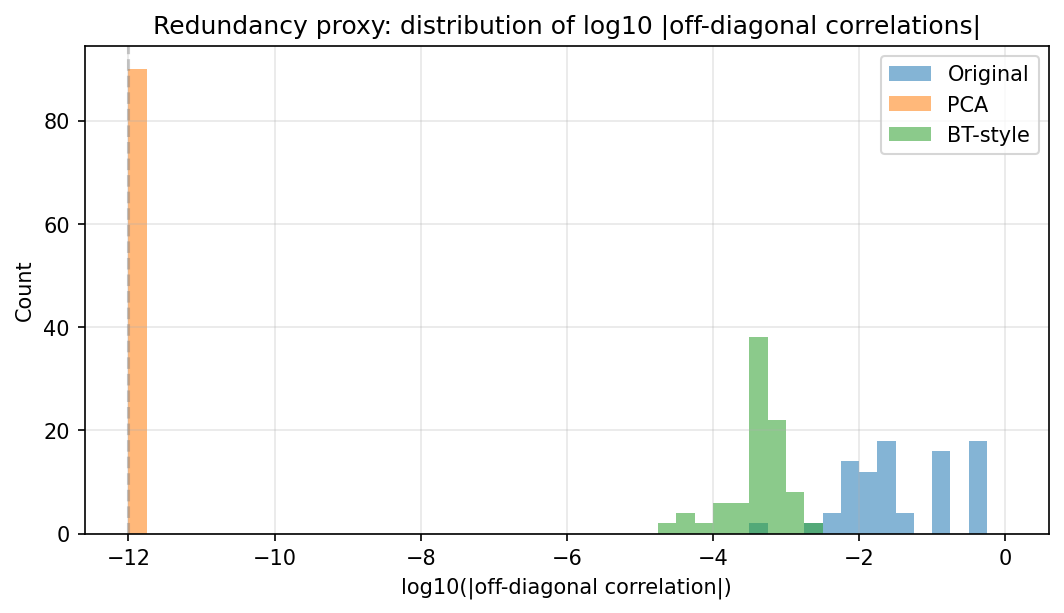
In Figure 2, PCA removes that redundancy post‑hoc by rotating the coordinates. The Barlow Twins‑style objective, in contrast, learns a transform so that cross‑view correlation is already close to identity.

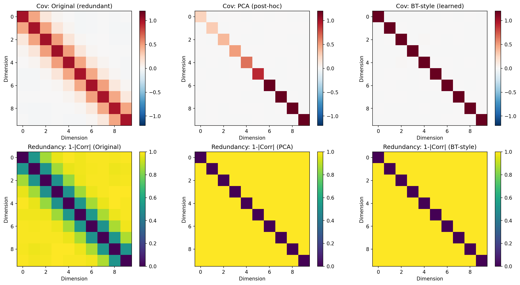
Covariance and redundancy maps: original (redundant), PCA (post-hoc), and Barlow Twins-style (learned)

Figure 2. Top: covariance matrices. Bottom: redundancy maps $1-\lvert\mathrm{Corr}\rvert$ (0 = redundant, 1 = decorrelated). Original (redundant), PCA (post-hoc), and Barlow Twins-style (learned).

The original representation exhibits structured redundancy between nearby dimensions. PCA removes this structure by rotation. Barlow Twins-style learning produces near-decorrelation directly, without an explicit post-hoc transform.

Distribution of absolute off-diagonal correlations showing redundancy reduction

Figure 3. Distribution of $\log_{10}(\lvert C_{ij}\rvert)$ for off-diagonal entries ($i\neq j$). PCA and Barlow Twins-style learning concentrate mass near zero correlation, so a log scale makes the shrinkage visible.

What this example does not show

This toy setup is intentionally narrow. It does not claim that Barlow Twins produces semantically better features than PCA, nor that decorrelation alone is sufficient for representation quality. The goal here is only to make the statistical role of the loss explicit.

Basis alignment

Barlow Twins-style learning isn’t “just decorrelating,” but it’s also not “finding the PCA rotation.” Because the constraint is defined across views, the solution is free to rotate the representation without changing the objective much once (\mathbf{C}) is close to the identity. That’s why it’s not meaningful to ask for “the” Barlow Twins rotation the way it is for PCA.

So the goal of this section is modest: to show that the learned coordinates don’t need to line up with PCA eigenvectors, even when the learned representation is comparably non‑redundant.

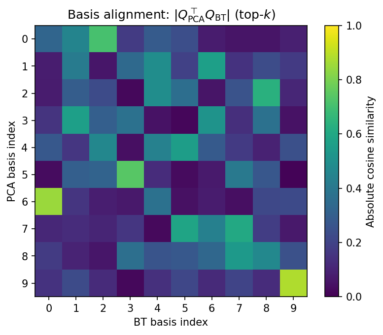
Basis alignment heatmap showing |Q_PCA^T Q_BT|

Figure 5. Basis alignment: absolute cosine similarities between PCA and Barlow Twins-style bases. If bases matched, this would be a permuted identity.

Because the constraint is defined across views, Barlow Twins is free to rotate the representation. The learned basis need not coincide with PCA eigenvectors.

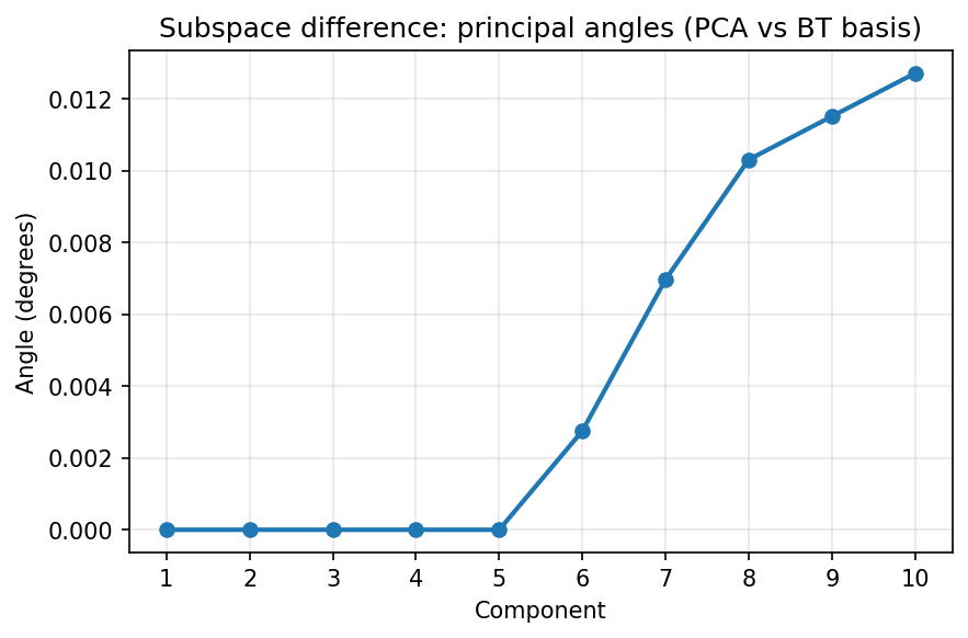
Figure 6. Principal angles between PCA and Barlow Twins subspaces. Small angles indicate similar subspaces; large angles indicate different orientations.

In this toy setup, the subspaces can be similar (small principal angles) while the coordinates differ. That’s exactly the non‑identifiability point above: Barlow Twins cares about correlation structure across views, not about matching a particular eigenbasis.

A Likelihood-Based View: Correlation Constraints vs Model Classes

The basis-alignment plots raise a natural question: if the coordinates are “free to rotate,” what is actually being constrained? One way to make that concrete is to switch lenses.

Correlation constraints (like Barlow Twins) and likelihood-based objectives operate under different assumptions. Below, I use a simple Gaussian likelihood diagnostic to show which parts are rotation-invariant (full covariance) and which parts depend on the chosen coordinate system (diagonal / isotropic).

Gaussian negative log-likelihood comparison under full, diagonal, and isotropic covariance assumptions

Figure 7. Gaussian negative log-likelihood (NLL, nats per sample) under three covariance assumptions: full (rotation-invariant), diagonal (basis-dependent), and isotropic (basis-dependent). Lower is better.

A useful way to sharpen the distinction is to ask a different question: if I pretend the representation is Gaussian, how well does it fit under different covariance model classes?

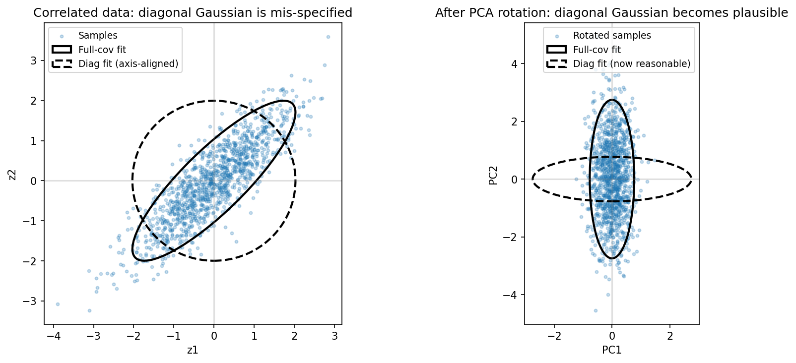
Full‑covariance Gaussian NLL is rotation‑invariant. Think of fitting a tilted ellipse to your data. If you rotate the paper, the ellipse still fits perfectly, the shape is what matters, not the orientation. Similarly, if you fit a Gaussian with full covariance by MLE, rotating the representation (e.g., PCA rotation) leaves the optimum NLL unchanged because $\log\det(\Sigma)$ is invariant under $\Sigma \mapsto Q^\top \Sigma Q$.

Diagonal / isotropic Gaussian NLL is basis‑dependent. Now think of fitting an axis-aligned ellipse (diagonal covariance) to tilted data. If your data is correlated (tilted), the axis-aligned ellipse fits poorly. You must either rotate the data to align with the axes (PCA), or force the network to produce data that is already axis-aligned (Barlow Twins). These model classes bake in stronger assumptions (conditional independence for diagonal; a single variance for isotropic), so the coordinate system matters.

Ellipse fitting analogy: full-covariance vs diagonal-covariance Gaussian likelihood

Visual analogy: full-covariance Gaussian fits a tilted ellipse (rotation-invariant); diagonal-covariance Gaussian fits an axis-aligned ellipse (basis-dependent). PCA rotation makes the diagonal fit reasonable.

Two important caveats:

This is a diagnostic on the representation distribution, not a likelihood for the original images. We’re changing the random variable when we rotate/whiten.
Barlow Twins is not trying to be Gaussian; it’s enforcing a correlation target across views. A worse Gaussian NLL is not a “failure”, it just reflects a different objective.

With that framing, Figure 7 is easy to read: full‑covariance NLL barely cares about rotations, while diagonal/isotropic NLL does.

Why this isn’t a generative model

Barlow Twins is not a generative model. It aligns augmentation-invariant information across views but does not learn a decoder or likelihood for reconstruction. Because Barlow Twins minimizes redundancy (off-diagonals) without explicitly maximizing the “volume” of the representation (like a VAE or flow model might), it creates a very efficient, compact code, one that doesn’t necessarily cover the whole space required for generation. The high NLL values we saw in Figure 7 reflect this: Barlow Twins optimizes for decorrelation, not for filling the latent space uniformly.

Summary

PCA: diagnose redundancy after learning, then remove it via an explicit, identifiable rotation (a change of basis).
Barlow Twins: impose a training-time correlation constraint; the learned basis is not unique once decorrelation is achieved.
$\lambda$: the knob that prices duplication, once it’s high enough, redundancy hits a floor and returns diminish.

References

Jure Zbontar, Li Jing, Ishan Misra, Yann LeCun, Stéphane Deny. Barlow Twins: Self-Supervised Learning via Redundancy Reduction. ICML 2021. arXiv:2103.03230.
Di Zhang. On the Optimal Representation Efficiency of Barlow Twins: An Information-Geometric Interpretation. arXiv:2510.10980 (submitted 2025).