Hangman with DQN and Transformers

TL;DR. We train a small bidirectional Transformer + Double DQN to play Hangman, restricted to words ≤5 characters (training and inference) to keep the demo clear and controlled.

• Two-stage: masked‑LM style pretraining (letter presence + next‑letter) → Q-learning with replay, target network, and Huber loss.
• Action masking guarantees we never re‑guess letters; optional dictionary-aware pruning further narrows choices.
• Guided exploration samples from the pretrained policy (temperature‑scaled) instead of uniform random; a small information‑gain reward encourages guesses that shrink the candidate set.
• Curriculum (2–3 → 4 → 5 → mixed ≤5) stabilizes learning.

Hangman is a great example of a reinforcement learning problem: we only see part of the word, make sequential guesses, and choose from a small set of actions (the 26 letters). Deep Q-Networks (DQN) fit naturally here because they handle discrete actions well and can learn to avoid invalid guesses through action masking.

RL Setup

In our RL setup, we model Hangman as an MDP $ M = (S, A, P, r, \gamma) $:

• Actions: The 26 letters of the alphabet, excluding those already guessed.
• State: Includes the current revealed word, guessed letters, remaining attempts, word length, and optionally a category.
• Transitions: Picking a letter reveals matching positions, updates the state, and reduces attempts if the guess was wrong.
• Rewards: We get positive rewards for revealing letters, $+10$ for winning, and $-5$ for losing.
• Goal: Maximize the expected sum of discounted rewards over time.

Example.
Suppose the hidden word is cat with 6 attempts:

1. Start: _ _ _, attempts = 6.
2. Guess e: wrong → still _ _ _, attempts = 5.
3. Guess a: correct → _ a _, attempts = 5.
4. Guess c: correct → c a _, attempts = 5.
5. Guess t: correct → c a t, win with bonus reward.

This illustrates how actions, states, transitions, and rewards are applied in practice.

Strategy at a glance. We play with a masked ε-greedy policy (only unguessed letters are considered), learn Q-values with Double DQN + Huber loss, and use a small curriculum (short → longer words). The Transformer encoder is pretrained to “fill the blanks,” then warm-starts the Q-head for RL.

RL Architecture: DQN with Transformer

Q-Learning Basics

Our agent learns a Q-function that scores each possible letter given the current game state. Action selection mixes exploration and exploitation: with probability ε it picks a random valid letter, otherwise it chooses the letter with the highest Q-value. To stabilize learning we use a target network and Double DQN updates. The target is:

where the maximization only considers unguessed letters. Training minimizes the Huber loss between these targets and predictions. For faster convergence, the Q-head can be initialized from supervised pretraining or simple heuristics.

Why Double DQN here?

Plain DQN uses the same network to select and evaluate the next action, which tends to overestimate noisy Q-values: \(y_t^{\text{DQN}} = r_t + \gamma \max_{a' \in A_{t+1}} Q_\theta(s_{t+1}, a').\)

In Hangman, that bias is amplified because:

• The action set is tiny (26 letters), so a single overestimated wrong letter can easily win the max.
• Many actions are effectively low-value (or invalid after masking), and a few bad picks end the episode quickly.
• Rewards are sparse and spiky (big win/loss bonuses), which makes target noise matter more.

Double DQN splits selection and evaluation to mitigate that bias:

Here, $\theta$ are the online parameters (updated every step) and $\bar{\theta}$ are the target parameters (updated slowly via periodic copies; see Training).

From Probabilities to Q-values

We may use two sources of “how likely is this letter?” information:

• (1) static frequency/co‑occurrence from the dictionary and
• (2) contextual probabilities from the Transformer, $P_{\text{ctx}}(a\mid s)$, which change with the revealed pattern.

These give a quick estimate of immediate gain, e.g., the expected number of positions a letter will reveal. While probabilities capture the likelihood of letters, Hangman’s rewards are delayed and shaped by wins/losses. Q-values fuse likelihood cues with discounted future return, aligning guesses with long-term success. The Q‑head then turns these signals into expected discounted return

balancing short‑term reveals, time penalties, win/loss bonuses, and information‑gain terms. In practice we warm‑start the Q‑head from the pretrained “next‑letter” logits or from a simple heuristic like

then let RL fine‑tune it with replay + target network.

Policy (what we actually execute)

The policy is derived from Q—not from raw probabilities. We act with a masked $\varepsilon$-greedy rule over the set of valid, untried letters $A_t$:

Thus, $\pi$ is not a softmax over probabilities but a greedy selection with exploration noise.

• Masking: once a letter is guessed, it’s removed from $A_t$. We optionally add dictionary‑aware masks to prune letters that are inconsistent with any remaining candidates.
• Guided exploration: when we explore, we can sample from the pretrained next‑letter head (temperature‑scaled) instead of uniform, which keeps exploration sensible without being greedy.

Because training is off-policy, even exploratory actions ($\epsilon$-greedy or guided) provide useful information for improving the greedy target policy.

Transformer Encoder

We encode the game state with a small bidirectional Transformer.

1. Inputs are (1) the partially revealed word and (2) a 26‑dim mask indicating already‑tried letters.
2. Bidirectional self-attention processes the entire sequence to estimate which characters fit each position, using context from both sides of each blank.
3. Mean‑pool the non‑pad tokens into a fixed vector and reuse it for two heads: supervised heads for presence/next‑letter during pretraining, and a Q‑head for RL.

In practice, the encoder turns contextual letter likelihoods into sharp action values, which makes Double DQN targets less noisy and learning more stable.

The online and target networks share the same architecture (Transformer encoder + Q-head) but keep separate weights. The target’s slower updates reduce overestimation noise while evaluating the online net’s greedy choice.

This specialization allows the model to develop different strategies for different types of letters, making it more effective at the sequential decision making required in Hangman.

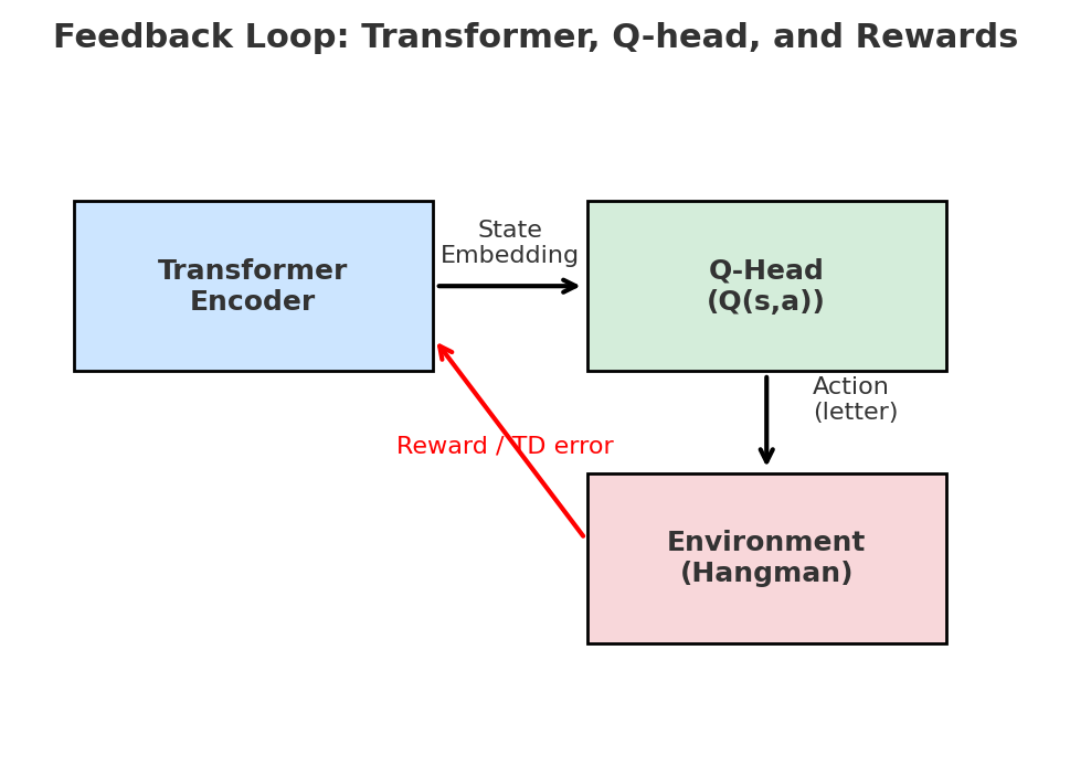
Feedback from Rewards

Although the Transformer encoder by itself just encodes context (e.g., which letters are visible, where blanks occur), the reinforcement signal backpropagates through it. When a guessed letter brings a negative reward (like a wrong guess penalty), the corresponding Q-value is pushed downward by the TD error. That gradient flows not only into the Q-head but also into the Transformer, tuning its representations so that it can better separate “good guesses” from “bad guesses” given the context.

This mechanism is what makes the setup model-free and off-policy:

• Model free: the Transformer never models transition probabilities explicitly — it just adjusts its embeddings so that Q-values align with observed returns.
• Off policy: the agent may explore with a behavior policy ($\epsilon$-greedy or guided exploration), but the Q-function is always trained toward the greedy target policy. Even “bad guesses” made under exploration provide useful gradients, because the TD error teaches the encoder which contextual features lead to long-term penalties vs. rewards.

For example, guessing z in _ a _ leads to a penalty, so the model learns to assign low Q for “z” in contexts like that, but not globally, since in pi_za the same “z” could be high-value. This is what makes the contextual Transformer embedding crucial: it lets the agent learn that the value of a letter is conditional on the current pattern, not fixed.

Experience Replay and Minibatch Training

To keep learning stable, we don’t update from sequential transitions directly. Instead we maintain a fixed‑capacity (FIFO) replay buffer that stores transitions of the form

As the agent plays Hangman, each transition is appended on the fly (not pre‑generated). During training we draw i.i.d. minibatches ${B}$ by uniform random sampling from the buffer. This:

• Breaks correlation between consecutive guesses, improving stability,
• Reuses data for better sample‑efficiency, and
• Supports off‑policy updates (we can learn a greedy target policy from exploratory behavior).

Given a minibatch ${B}$, we compute the Double DQN target as defined above (with action masking in the next state), and minimize the Huber loss:

In practice we also wait for a small warm‑up (e.g., a few thousand transitions) before starting gradient updates, so early noisy experiences don’t dominate training.

• Breaks correlation: Sampling out of order avoids the instability of updating on consecutive, highly correlated moves.
• Improves data efficiency: Each past experience can be reused multiple times in different minibatches.

These minibatches are then used to compute Double DQN targets and update the Q-head. In practice, this means the Transformer encoder and Q-head learn from a diverse set of examples in each update, smoothing learning curves and reducing variance.

Implementation

The core architecture combines character embeddings with positional and length information:

class CharTransformer(nn.Module):
    def __init__(self, d_model=128, nhead=4, nlayers=2, max_len=35):
        super().__init__()
        # Core embeddings
        self.emb = nn.Embedding(VOCAB_SIZE, d_model, padding_idx=PAD_ID)
        self.pos_enc = nn.Embedding(max_len, d_model)
        self.len_emb = nn.Embedding(max_len + 1, d_model)
        self.tried_proj = nn.Linear(26, d_model)  # A–Z one-hot → d_model
        # Encoder
        enc = nn.TransformerEncoderLayer(d_model, nhead, d_model * 4, dropout=0.0,
                                         batch_first=True, norm_first=True)
        self.transformer = nn.TransformerEncoder(enc, num_layers=nlayers)
        # Heads
        self.sup_heads = SupHeads(d_model)  # pretraining
        self.q_head = None                  # added for RL
    def add_q_head(self):
        self.q_head = DuelingQHead(self.d_model)

Training

We trained on a dictionary of ~227k English words, filtered by length to create a curriculum of stages. The idea was to let the agent tackle easier cases first (short words) before moving to harder ones.

For demonstration purposes, we restricted both training and inference to words of length ≤5.

Two-stage learning:

1. Supervised pretraining. The Transformer is warmed up with “fill-the-blank” objectives: predicting which letters are present and which one comes next, given partially masked words. This produces millions of cheap training samples and gives the model a strong starting point.

2. Q-learning fine-tuning. The Q-head is added and trained with Double DQN, replay memory, Huber loss, and a target network.

Action selection uses a masked $\varepsilon$-greedy policy: with probability $\varepsilon$ the agent samples a random valid letter, otherwise it chooses the letter with the highest Q-value. Already guessed letters are always excluded.

Stability tricks

• Freeze the encoder for early RL, then unfreeze.
• Lower LR for the encoder, higher for the Q-head.
• Gradient clipping (1.0) and periodic target updates.
• Optional dictionary-aware masking to prune impossible guesses.

Curriculum learning moves from 2–3 letter words → 4 letters → … → N letters → mixed up to N.

This keeps training stable and prevents the agent from collapsing into random guessing when faced with long words too soon. At the end of each stage, we test on held-out words, reporting solved rate, average reward, and number of guesses.

Results & Analysis

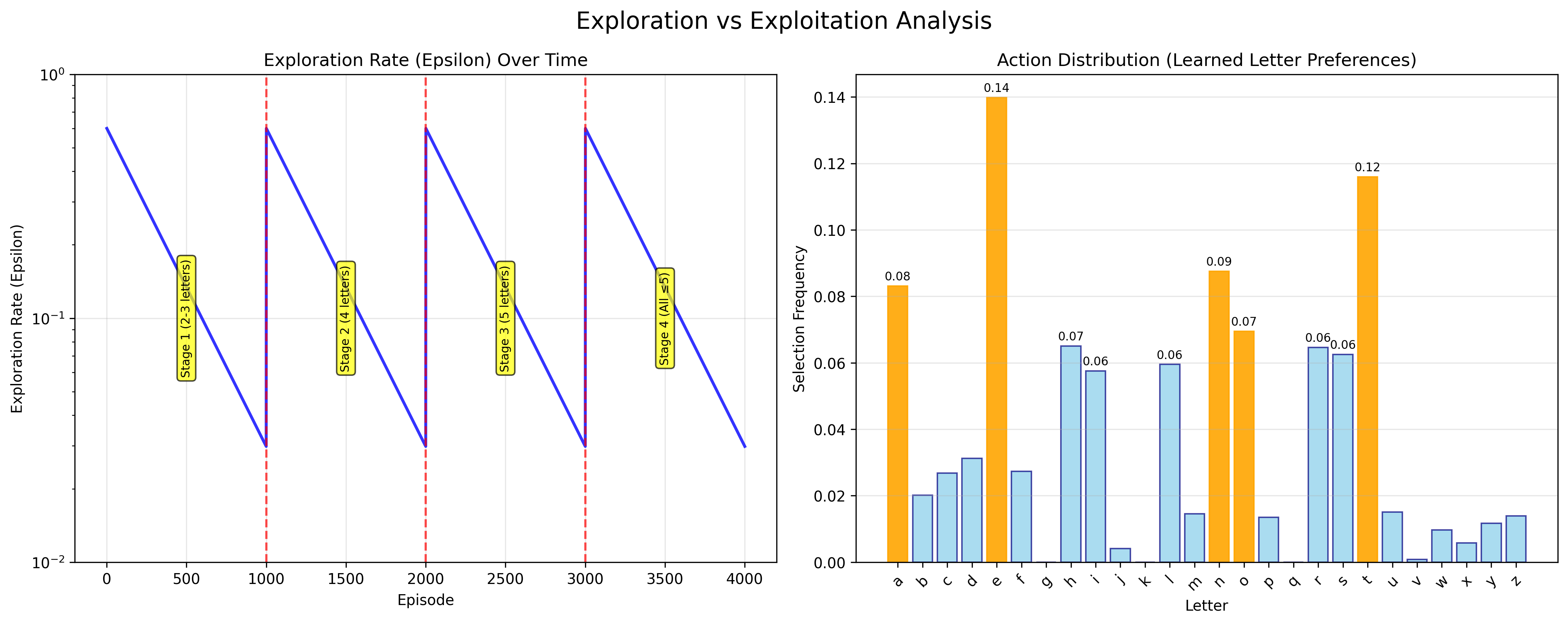
The plots below summarize how the agent improves over training and how exploration balances against exploitation.

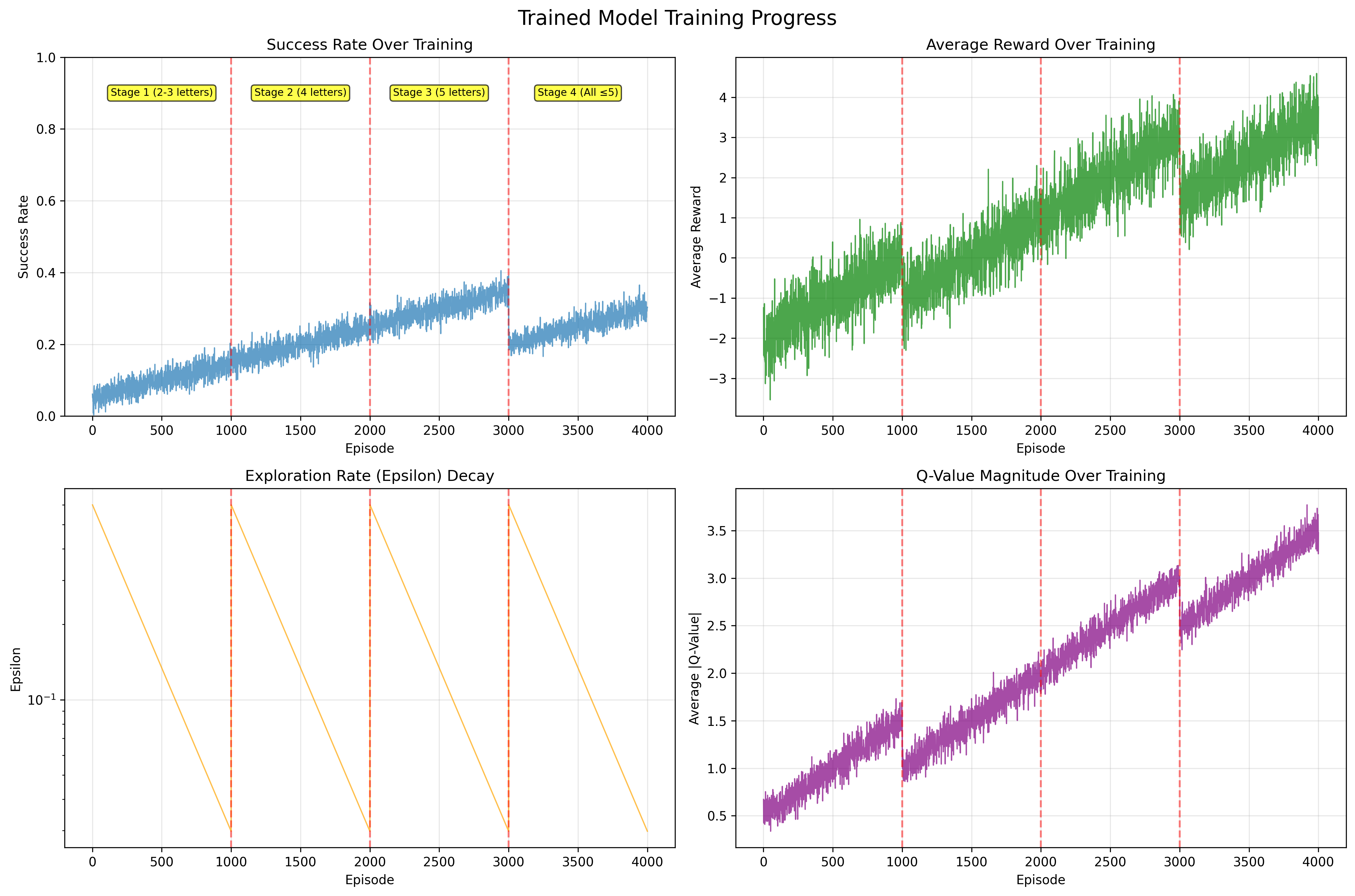
Key findings:

• Curriculum learning enables stable progression from short to longer words, preventing random guessing collapse
• Reward shaping accelerates learning and stabilizes Q-value estimates through proper scaling
• Exploration balance with ε-greedy decay provides early exploration while converging to strong exploitation
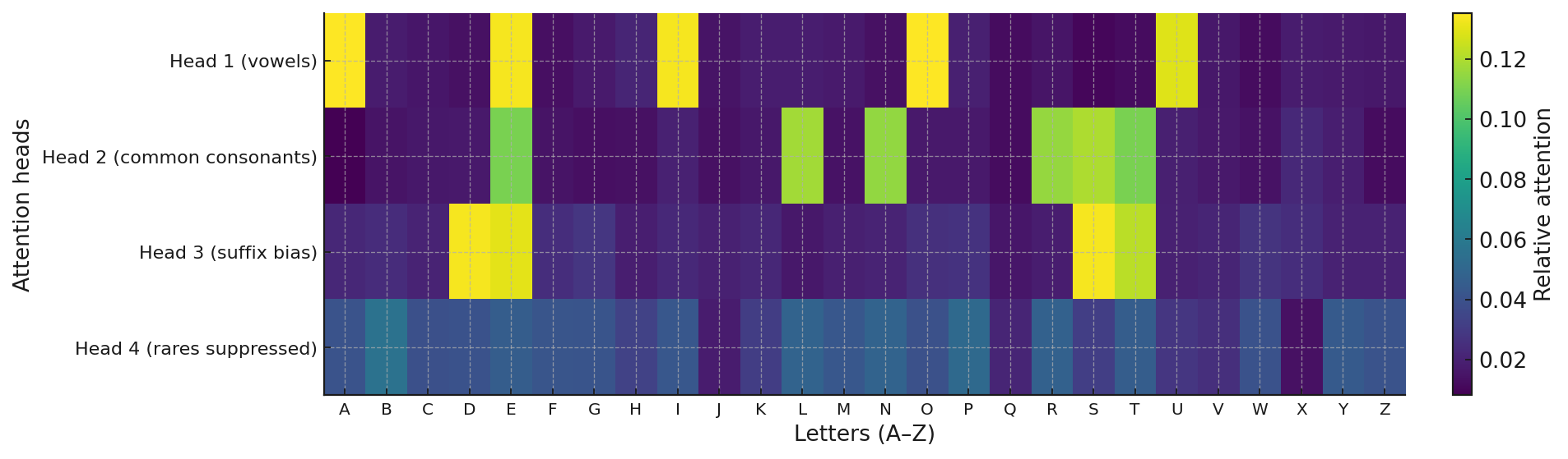
• Attention specialization reveals heads focusing on different character groups (vowels, consonants, suffixes)

Inference: Agent Playthroughs

To better understand how the trained agent makes decisions, we visualize its behavior on specific words. Below are two examples (house and light), showing how Q-values, attention signals, and action choices interact over the course of a game:

• Q-values: The bar chart shows the Q-value assigned to each letter. Already-tried letters are masked (red), and the chosen action is marked in green.
• Top letters: The model highlights the highest-value letters, with the chosen one (i) among them.
• Attention scores: Attention heads assign high scores to vowels like u and i, reflecting strong prior knowledge of English word structure.
• Decision rationale: The correlation plot shows how Q-values align with attention-based likelihoods. The agent selected i with a modest Q-value but reasonable attention support.

Example 1: Word = house

Example 2: Word = light

Takeaway: Even if the top attention signal does not correspond directly to the selected letter, the Q-function steers the policy toward actions that maximize long-term reward.

Conclusion

• The Transformer encoder supplies strong contextual priors via attention, often highlighting vowels and frequent consonants as promising candidates.
• The Q-head integrates these priors with reinforcement signals and enforces explicit action masking, ensuring that once a letter has been tried or ruled out by dictionary constraints, its probability is zeroed in subsequent steps.
• This design allows the agent to update conditional likelihoods dynamically as the game evolves, rather than reusing failed guesses, leading to more reliable strategies than simple frequency heuristics.