ZK State Prune: The Boundaries Behind Rollup Cost Models

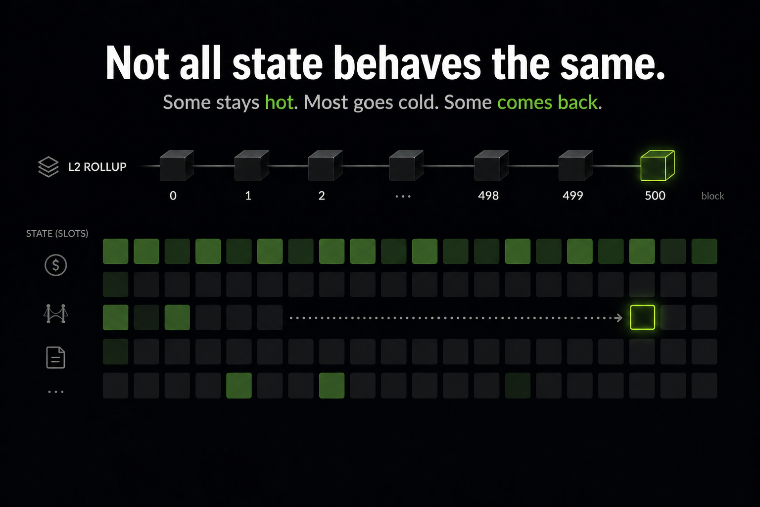
L2 rollup state slots over 500 blocks: hot slots (in memory), cold slots (in storage), accesses (hits in memory), and reactivations (cold misses) — different slots show different lifecycle patterns

Not all state behaves the same. Some stays hot. Most goes cold. Some comes back.

A user bridges USDC onto a rollup. The balance slot gets touched, updated, then sits idle for hours. Another transaction arrives later and touches it again. Meanwhile, thousands of other slots in that block were touched once and never used again.

A rollup node has to decide: which of these stays in fast memory, and which can move to a slower tier?

That is the hot/cold state problem. The hard part is that “old” is not the same as “dead.” A slot can sit idle for a long time and then be accessed again. If the system demotes it too early, the next access becomes a cold miss; if it keeps too much state hot, the node pays unnecessary memory and lookup cost.

This looks like a caching problem. It is — except the cost of getting it wrong shows up as latency, proof size, and node hardware requirements in a rollup.

The previous post argued that this should be treated as a prediction problem: estimate the probability that a slot will be reused within a future horizon, then turn that probability into a cost-aware tiering decision.

The first version of zk-state-prune implemented that idea as a Go pipeline:

extract state-access data (RPC / statediff)
fit a survival model
simulate hot/cold tiering policies
print a cost table

It worked. And that was the problem.

The numbers looked precise. But I had no way to answer the basic questions a downstream reader would ask:

What exactly did the extractor observe?
Were two runs actually comparable?
Did a “win” come from the model, or just from a smaller RAM budget?
Was a result stable, or just a lucky window?

At that point, the issue was no longer the model. It was that the artifact had no clear boundaries. The predictive policy decides when to demote; the guardrails name the boundaries under which that decision is valid.

What the pipeline actually sees

Before talking about guardrails, here is what the pipeline sees on real data — three slots from a 100k-block window on Scroll mainnet, captured via public JSON-RPC eth_getLogs on Transfer events, evaluated under the same 50-block hot/cold threshold used in the synthetic figure from the previous post:

Three real Scroll slots over 500 blocks under a 50-block threshold: heavy hitter stays hot, reactivating slot is demoted then re-promoted, one-shot slot is demoted after the first event

Three real Scroll slots from the scroll_100k run under a 50-block threshold. Top: a system-contract slot with 87 events stays hot throughout. Middle: a holder slot with a 389-block gap gets demoted at block 91, then re-promoted (★) at block 430. Bottom: a one-shot slot demoted 75 blocks after its single event.

The reactivation star on the middle lane is the kind of thing the system has to be honest about. The data source here is the RPC Transfer-log surrogate — the timeline is what was visible to the extractor, not the full state-access surface. There may be more reactivations in reality (reads, non-Transfer writes the surrogate cannot see). If that distinction is not machine-readable in the artifact itself, downstream readers will quote the figure as the full picture.

What the model is actually estimating is $p_i(\tau)$: the probability that slot $i$ will be accessed again within horizon $\tau$.

The prediction target p_i(τ) = P(T_i ≤ τ | T_i > t_0, x_i), with annotations: T_i ≤ τ means not accessed within τ, T_i > t_0 means observed alive at t_0, x_i means features of the slot. Footnote: survival analysis with right-censoring, time truncation, and partial observability.

That estimate is built on history that is censored (some slots are still alive at the end of the window), truncated (the window starts mid-life), and partial (the extractor only sees part of the access surface). The guardrails below exist because the gap between what $p_i(\tau)$ assumes and what we actually observed is structural — not a bug we can fix in the model.

The boundaries behind a cost number

As rollups scale and push more execution off-chain, the gap between what is observable and what actually happens only gets larger. That makes this kind of domain confusion more likely, not less.

The guardrails that ended up in the pipeline were not in the original design. They were forced in — every one exists because there was a concrete way the system could mislead me, or someone else, without it.

The shape of those constraints is familiar to anyone who has worked on blockchain systems:

Domain separation. A signature is only valid under a specific context (chain id, contract, nonce, intent). For a cost table: a metric must be bound to the observation domain that produced it.
Replay protection. The same input cannot be reused under mutated assumptions. For a cost table: a --resume run cannot mix two different filtering regimes into one database.

The pattern is well-known in production. After the 2016 DAO fork, the same signed Ethereum transaction could be replayed on both ETH and ETC because transactions were not yet bound to a chain ID. That was a domain failure, not a cryptographic one — and a --resume run without domain binding is the same bug shape in a different system.
Partial observability. Not all state transitions are visible from a given interface. For a cost table: “not visible” is not “absent” — the extractor has to declare what it can and can’t see.
Tail / adversarial mindset. Average-case OK is not enough; the worst case is what releases.

A cost table without its observation domain is no different from a replayable transaction: the same bytes interpreted under unrelated assumptions.

The four boundaries I had to draw

Each guardrail came out of a concrete moment the pipeline almost lied to me, and the boundary that moment forced into the artifact.

1. Capability stamps — what the extractor can see

The RPC Transfer-log surrogate and the state-diff extractor write the same schema — state_slots, access_events, the same Cox fit, the same zksp report. But they see different worlds. The surrogate sees Transfer-derived pseudo touches only: no reads, no non-Transfer writes. The state-diff extractor sees the full read-and-write surface. Same database file, same chart, two completely different observation domains. If both artifacts land in the same sweep, the chart is silently comparing different observation processes.

The fix: every extractor implements a Capability interface that declares what it observes — source, observes_reads, observes_non_transfer_write — written into schema_meta at the end of extraction. Downstream consumers banner-print it, surface it in JSON envelopes, and refuse to mix artifacts whose stamps disagree. qa_viz.py treats a data_source mismatch as a hard fail, not a warning.

The boundary becomes machine-readable: the artifact tells you exactly which lifecycle it has observed.

2. Extract limits — what the extractor filtered out

One block in the 100k-block Scroll run emitted 218 access events, roughly 50× the median across active blocks. That may be legitimate chain activity (token launch, airdrop), or it may be an RPC / ingestion failure. Same shape, very different meaning for a survival fit. Letting an unbounded block mutate the database first and asking questions later is the wrong failure mode for an analysis pipeline.

The fix: opt-in per-block hard limits, calibrated from the observed run with conservative headroom (thresholds and rationale in EXTRACT_LIMITS.md). The extractor pre-tallies each block before writing any rows; if a tally exceeds its limit, it fails closed rather than silently truncating. The chosen limits land in schema_meta as a second stamp, extract_limits. A --resume run that arrives with different limits is rejected.

Two stamps in one mechanism: data_source for coverage, extract_limits for filtering, both stored as JSON values in schema_meta

Two domain-binding stamps in the same key/value table — coverage and filtering, both stored as JSON values the extractor controls and downstream code can refuse to ignore.

3. Same-RAM matching — what is actually being compared

I kept comparing policies and getting “wins” that made no sense. The statistical policy at miss penalty $\ell = 32$ looked good on TotalCost, but it kept only 0.04% of slots hot and caught 18.8% of accesses — it had not learned a useful placement rule; the cost parameters had pushed it into a degenerate corner. It turned out I was just comparing different RAM budgets: a smaller hot set always implies smaller RAMCost.

The fix: only compare policies at the same RAM band (auto-pair only policies whose RAMRatio differs by less than ε), and flag degenerate cells (kept-few + pruned-most + miss-heavy) so they can’t drag a chart’s eye. With the apples-to-oranges hazard removed, what’s left is a real difference — not an artifact of the RAM budget.

4. Drift / out-of-distribution (OOD) — whether the past still describes the future

A tiering policy is a forecast. The honest validation is time-ordered: fit on a train window, evaluate on a future test window, repeat across rolling folds, measure the tail. For each fold the simulation also searches for a fixed-N baseline whose RAMRatio matches the predictive policy’s — otherwise we are back to the same-RAM problem above.

On the 100k-block Scroll rolling backtest, the all-fold mean was only mildly bad. The tail was not. For each fold, regret is TotalCost_statistical − TotalCost_matched-fixed — negative means the predictive policy wins:

Bar chart of max regret across 15 rolling folds: all_folds shows +487,075 (predictive policy loses badly), in_distribution shows -6,730 (predictive policy quietly wins)

Same backtest, two scopes. The 13 OOD folds make the tail catastrophic; the 2 in-distribution folds quietly win.

The two scopes disagree because a drift guardrail is doing its job. The backtest script compares train and test workload summary stats per fold; if any ratio exceeds --drift-ratio (default 1.5×), the fold is flagged out-of-distribution. On this run, 13 of 15 folds trip that flag.

The useful boundary is not “the model wins” or “the model loses” — it’s the artifact distinguishing the model is bad here from this is a different distribution. Three opt-in release gates (--max-regret, --min-coverage, --max-fpr) wrap that distinction in a CI exit code, so a regression in policy quality and a regime shift can be told apart.

What this does not claim

The motivation is real failure modes that show up in L2 systems (DoS-like endpoint instability, schema drift, tail behaviour under workload shifts). It is not a protocol-security analysis.

Covered. Endpoint / ingestion robustness, domain-binding via stamps, out-of-sample policy evaluation, tail-risk surfacing.
Not covered. Censorship-resistance guarantees, data-availability guarantees, bridge / fund-security vulnerabilities, “L2 attacks” as a comprehensive taxonomy.

If you quote a number from a zksp run, record five things:

Chain + window [start, end) and the run command
data_source capability stamp (rpc vs statediff)
Cost parameters: ram_unit_cost, miss_penalty, tau
Stamped extract_limits and the extractor endpoint
Repo commit SHA

Closing

A rollup node never sees the full lifecycle of its state. It sees a projection of it — shaped by the extractor, filtered by limits, summarized into a cost table. The model makes a prediction on that projection. The artifact turns that prediction into a number.

The question is not whether the number is correct. It is whether the number knows what it is.

A predictive system does not fail only when the model is wrong. It fails when it produces numbers under assumptions the artifact never names.

A cost number is only useful when its boundaries are named.