Ethereum Gas Changepoints Are Warning Signals, Not Regime Labels
An empirical diagnostic pipeline for fee-risk stress testing under EIP-1559.
TL;DR. Gas changepoints are useful as warning signals, not regime labels. In this 100k-block window, raw detector hits are strongly shaped by the spacing rule, so the useful output is a short ranked list of fee-risk neighborhoods. The strongest candidates are mostly fee-level shifts with nearly flat utilization, which makes them useful for stress testing but weak evidence for clean demand-regime breaks.
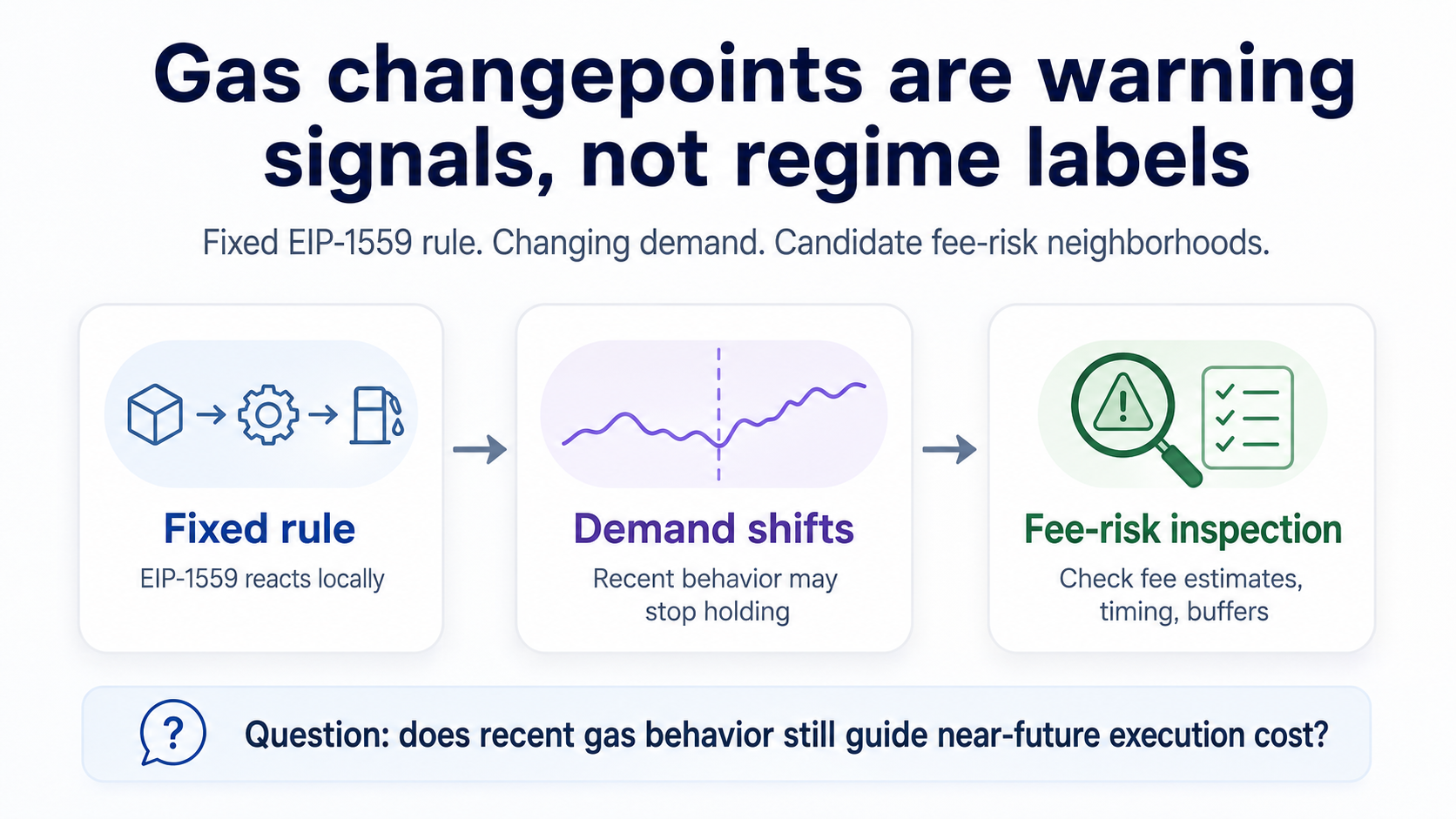
Under EIP-1559, the update rule is fixed; the demand feeding into it is not. EIP-1559 belongs to a narrower category than most macro-shock or governance-change stories: a fixed protocol feedback rule reacting to a changing demand process. This post uses changepoints as candidate neighborhoods for fee-risk stress testing—places where recent fee behavior may stop being a reliable guide for near-future execution cost—not as labels for gas regimes.
Why this matters
Wallets, bots, liquidators, and keeper systems all rely on short-horizon assumptions: recent base fees, recent utilization, recent volatility, recent inclusion conditions. Under EIP-1559, the update rule is fixed—but the demand process feeding into it can shift quickly. A local transition is therefore a natural place to stress-test whether fee estimates, execution timing, liquidation buffers, or oracle cadence assumptions still hold.
Changepoints are not tradable signals and not automatic regime labels. They are candidate neighborhoods where the recent-history assumption deserves extra scrutiny.
EIP-1559: a fixed rule reacting to a changing process
EIP-1559 replaced Ethereum’s first-price auction with a protocol-guided feedback system. Each block carries a base fee: a protocol-set reserve price on gas every included transaction must pay. If the previous block used more gas than the target, the next base fee rises; if less, it falls. The rule is fixed, deterministic, and local.
User tips (priority fees) are a separate layer; this note follows the protocol feedback path (base fee and utilization relative to target), not bidding behavior.
The feedback rule, explicitly
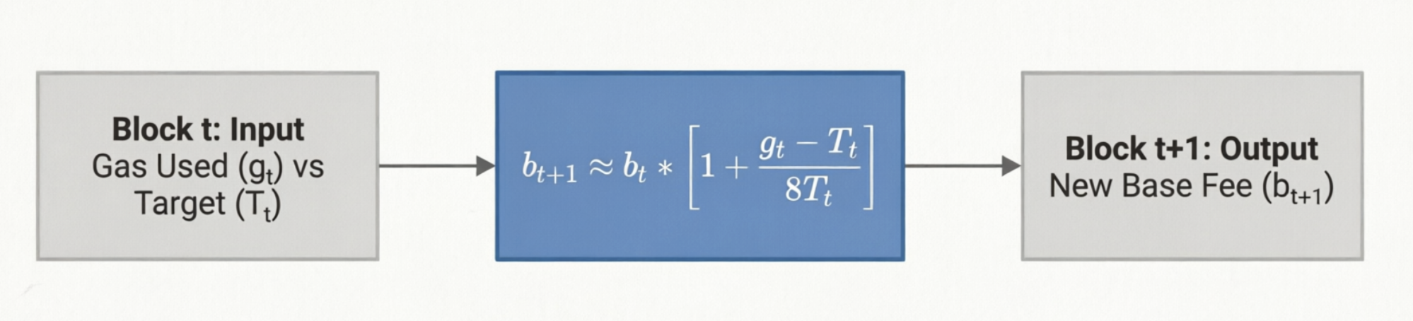
Let $g_t$ be gas used in block $t$, let $T_t$ be target gas for block $t$, and let $b_t$ be the base fee for block $t$.
Ignoring integer-rounding details:
\[b_{t+1} \approx b_t \left[ 1 + \frac{g_t - T_t}{8T_t} \right].\]The denominator 8 is EIP-1559’s adjustment-rate parameter: it limits the next-block base-fee change to roughly ±12.5% under the elastic block range. Above-target blocks push the next base fee up; below-target blocks push it down.
The controller reacts to realized demand; it does not forecast it. Uncertainty lives in the demand process feeding into it, not the rule itself.
I track three block-level signals:
- utilization_ratio = gas_used / target_gas — demand pressure seen by the controller.
- base_fee_gwei — the price level produced by the controller.
- base_fee_return = log 𝑏ₜ − log 𝑏ₜ₋₁ — short-horizon movement in the fee path.
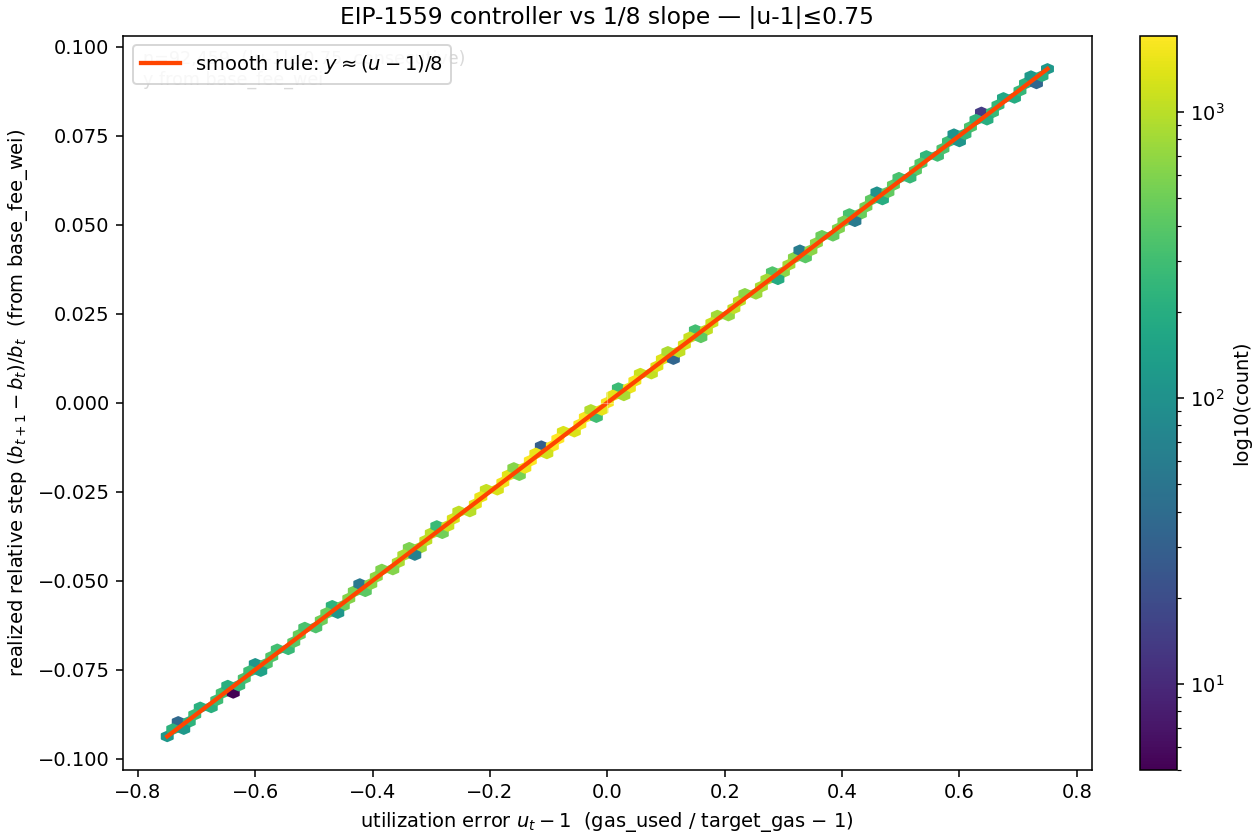
I use CUSUM as a changepoint screen: a way to flag candidate shifts in a time series, not a proof that a new economic regime began. It uses log_base_fee as a scale-stable view of the same price state; utilization and return enter as the other two block-level signals. The controller hexbin—a density plot for many overlapping points—uses the realized relative step $(b_{t+1}-b_t)/b_t$, because that is the quantity directly implied by the update rule.
The mechanism is fixed; demand is not
EIP-1559 updates locally, but we often summarize globally. The same fixed controller sees quiet blocks, short bursts, and sustained congestion; averaging over a whole window blurs those different local conditions.
Utilization is the controller input, base fee is the controller state, and short-horizon fee return is the controller’s immediate movement. The question is not where gas got momentarily expensive. It is:
When local demand pressure changes, how does the same block-by-block base-fee update rule show up in fee level, utilization, and short-horizon volatility?
I use changepoints as pointers, not labels. They tell me where to look; they do not tell me what the economy “was.” The follow-up is whether those neighborhoods show coherent, persistent shifts or mostly configuration-shaped detector output.
Everything here is block-level and conservative, not a mempool or transaction-level story.
Where this sits
This post is narrower than prior work on EIP-1559 mechanism design and fee dynamics: it focuses on how to read local block-level diagnostics without turning detector output into regime claims.
What we found (substance first)
1. Mechanism reconstruction checks out
On the recent 100k-block window, EIP-1559 reconstruction is exact in the audit sense used here: zero invalid intervals, zero max absolute error in wei. The adjacent 100k-block window passed the same audit, but what repeated across both was detector behavior under the same spacing rule, not a clean economic story. Every downstream ratio or delta is conditional on that fee path being right.
| Metric | Value (recent window) |
|---|---|
| Validation intervals | 100,000 |
| Invalid count | 0 |
| Invalid rate | 0.000000 |
| Max abs error (wei) | 0 |
2. The window itself is “busy” in a useful way
The recent window is contiguous and busy enough to stress-test local fee behavior:
| Metric | Value |
|---|---|
| Rows | 100,001 |
| Block range | 24,951,126–25,051,126 |
| Missing blocks | 0 |
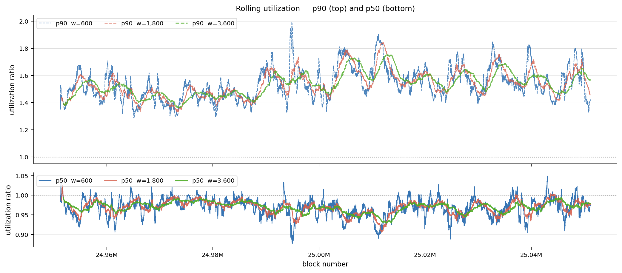
| Utilization p50 / p90 | 0.9711 / 1.5367 |
| Base fee gwei p50 / p90 | 0.318799 / 1.789423 |
| Gas-limit changes | 33,338 |
| Above-target rate | 0.463 |
The gas-limit and above-target rows are rounded for the table. The detailed breakdown is available from the local profile artifacts for this run (e.g., data/data_profile.md / data/profile.json) in the repository.
Roughly 13.9 days of wall time; ~46% of blocks are above target gas. Gas limit is not static wallpaper: this window contains 33,338 block-to-block changes across 46 distinct values—enough to log as a potential confounder. Any fee narrative should separate demand pressure from capacity movement.
Rolling utilization confirms the p50 / p90 split in the table: the median stays close to target across the window, but the upper tail remains elevated and bursty. That gap is why fee level can shift substantially while median utilization looks nearly flat.
3. Raw detector output is dense—and much of that density is structural
With min_distance=1200, a 100k-block window can hold at most roughly 83 non-overlapping hits. The three series produce 77–78 hits each. That is too close to the geometric ceiling to read as “78 regimes.”
Cross-series alignment has the same problem. Within ±1200 blocks, all three series appear perfectly aligned—alignment share = 1.0. But a spacing-preserving null baseline produces the same 1.0 alignment. Neighborhood alignment under this geometry is uninformative; I do not treat it as evidence of coordinated economic breaks.
Same-block overlap is the stricter check, and it is nearly absent: 0, 0, and 1 coincident hits across the three series pairs. The raw hit map is useful for proposing candidate neighborhoods, but it cannot carry the economic interpretation on its own. The sensitivity report in the repository makes the same point from another angle: hit counts move strongly with min_distance, so raw detector density should be treated as configuration-shaped.
4. A second stage is where the analysis actually lives
A high detector score does not guarantee a human-visible break. The interpretive layer asks:
- Did median and tail fees move by meaningful ratios across a fixed pre/post window?
- Did utilization / above-target / near-full behavior shift in the same direction?
- Did volatility step, and did the step persist at short post-horizons, or decay like a burst?
Candidates that pass explicit magnitude gates are ranked by an interpretability score, not by raw detector score. Most raw hits do not survive those gates. The object worth arguing from is the short ranked list and its local plots.
Three representative candidates show the pattern:
-
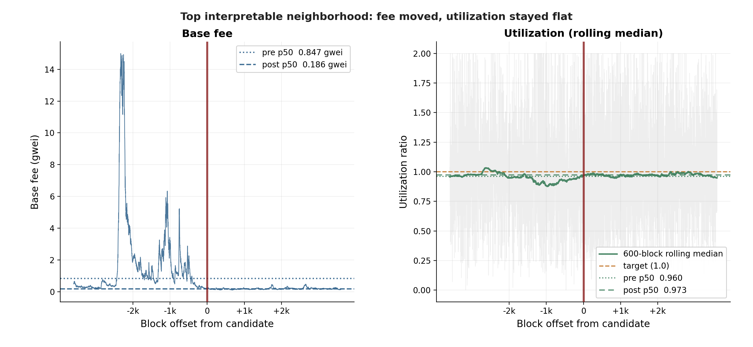
Block 24,995,644 — fee-level shift
Base fee p50 moved from 0.847 to 0.186 gwei, while utilization p50 moved only from 0.960 to 0.973. Persistent. -
Block 25,041,597 — fee-level shift
Base fee p50 moved from 0.160 to 0.866 gwei, while utilization p50 moved from 0.967 to 0.993. Persistent. -
Block 24,992,042 — volatility shift
Base fee p50 moved from 0.424 to 0.847 gwei, while utilization p50 barely moved from 0.956 to 0.960. Unclear persistence.
The top-ranked hit, block 24,995,644, is a persistent fee-level decay with only a modest utilization nudge—not a clean demand-regime break. Block 25,041,597 shows utilization moving more visibly, but the label remains fee-level shift. Block 24,992,042 is more instructive: volatility steps up, but persistence is unclear. That split is exactly why the second stage exists.
The broader pattern is the important part. In the full top-10, the strongest local candidates are mostly fee-level shifts with nearly flat utilization medians: fee moved 3–8× while utilization p50 shifted by 1–2 pp or less. That makes them useful fee-risk neighborhoods, but weak evidence for discrete demand regimes. The fee path and the controller input are not moving together cleanly in these cases.
Figures on the recent window
Mechanism check (not changepoints): a hexbin of utilization error $u_t-1$ vs. realized relative fee step $(b_{t+1}-b_t)/b_t$ on consecutive blocks (computed from integer base_fee_wei, same path as QA), with the smooth-rule line $y \approx x/8$. Integer rounding and the upward max(Δ,1) branch show as scatter off the line—especially near zero.
Where do those candidates sit in the full 100k-block window? The path below shows the global fee context—burst, decay, and spike structure—with the top interpretable candidates marked.
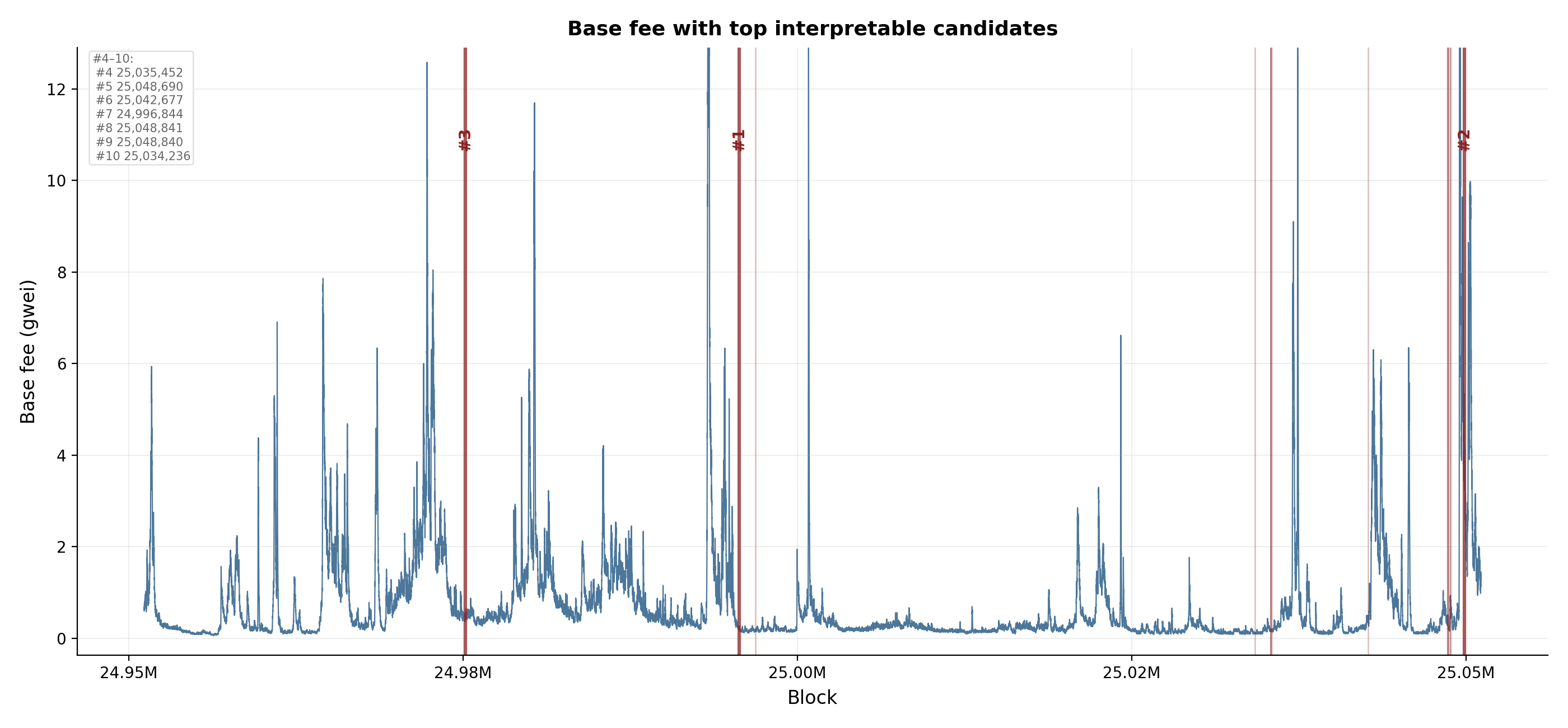
The top interpretability-ranked candidate (block 24,995,644) is the clearest local case: base fee decayed 4–5× while utilization p50 shifted by roughly 1 pp. The event card below shows all three signals across the pre/post window.
If you also look at detector-ranked panels (not shown here), expect mismatch: loud scores with weak local structure are in large part why the second stage exists.
What this means
The useful artifact here is not a regime map; it is a ranked stress-test queue. Raw changepoints are strongly shaped by the spacing rule; after null checks and local effect inspection, most hits look configuration-shaped rather than regime-like. What survives is a short list of neighborhoods where fee-level or volatility behavior shifted and persisted—the places to stress-test fee estimation, execution timing, and liquidation buffer assumptions. Whether those neighborhoods reflect real demand-regime breaks is a separate question. The broader point: feedback-controlled systems need diagnostics that separate candidate shifts from detector geometry.
Operationally, that queue marks where wallets and fee estimators might widen short-horizon buffers, where searchers and keepers might shorten refresh cadence, and where liquidation systems should re-check cost assumptions—not as proof demand entered a new regime, but as the places where the recent-history assumption is most worth questioning.
This is still a narrow block-level study: no mempool layer, no transaction-level bidding behavior, and only two adjacent 100k-block windows. But the audit trail matters: the EIP-1559 reconstruction is exact, detector saturation is visible, and the surviving candidates are inspected through local fee, utilization, and volatility behavior rather than raw changepoint scores. Some high-score points remain unclear after persistence checks—that is a finding, not a gap.
Appendix: reproduction context
Data: Ethereum mainnet blocks via JSON-RPC, two adjacent 100k-block windows (24851126..24951125 and 24951126..25051126). Detector: CUSUM window 7200, threshold 3.0, minimum spacing 1200. Local interpretation: 3600-block pre/post windows, persistence checks at +600 and +1800 blocks.
Diagnostics checklist, audit reports, and full ranked results are in the repository.