A Large DEX Order Is a Sequential Control Problem
Earlier posts isolated pool mechanics, dynamic fees, and liquidity response. This study uses the same lab for a different question: how to execute a parent order after each slice changes the market.
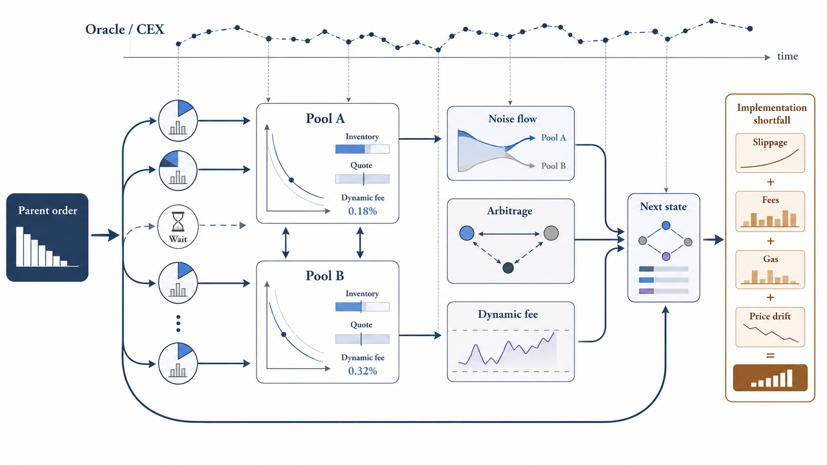
amm-lab/src/sim. A parent order is sliced across two competing pools; noise flow, arbitrage, oracle movement, and dynamic-fee updates then shape the next execution state. Conceptual schematic—not live-chain telemetry.
Every slice rewrites the next quote. A large DEX order is not one trade stretched over time; it is a sequence of decisions over the market state it creates.
I built a closed-loop DEX simulator with two competing pools, an external reference market, noise flow, arbitrage, and dynamic fees. The execution problem is to finish the remaining inventory when each slice changes the state faced by the next one.
What each slice changes
The task is to buy 50 units of the risky asset over 50 one-minute steps, equal to 5% of each pool’s initial risky-asset reserve. Every policy uses the same forced-completion rule: residual inventory is executed at the terminal state.
Each action changes several parts of the next decision. Routing selects between two evolving constant-product curves. The trade moves reserves and therefore the next marginal quote. The external reference price continues to move, while arbitrageurs can remove a favorable gap before the trader uses it. The controller may route to either pool, split the trade, or wait, but delay risks a more expensive terminal execution.
Fees follow an equilibrium-inspired linear rule in own inventory, rival inventory, and oracle misalignment. The rule is based on work on dynamic-fee competition between DEXs, where the switching boundary depends on both the oracle and rival exchange rates. I use that structure to close the simulated market, not to claim that the simulator solves the paper’s approximate Nash equilibrium.
The objective is implementation shortfall relative to the arrival price. This turns execution into a sequential control problem: the policy must price current cost against the state left for the remaining order.
Why historical swaps cannot answer it
Executed swaps are invaluable for calibration. They cannot support sequential execution learning because the replayed agent’s actions do not change the next pool state.
The tape does not show what would have happened if the trader had waited, split differently, routed elsewhere, or changed the next fee state. I tried historical replay across four data regimes. Apparent adaptive headroom disappeared under pre-specified audits because the recorded transitions did not respond to the replayed action.
The protocol-fee event study reaches the same boundary from the causal side. Trader-facing fees do not vary in that historical shock, trader types are latent, and the router’s full choice set is unobserved. The design identifies a liquidity-supply response, not a trader-routing counterfactual.
The matched event study detects no large short-run average withdrawal of active liquidity or local depth after LP take-rates were cut. That supports frozen depth as a short-horizon baseline, while leaving longer-run LP response open.
The benchmark is not TWAP
Production systems already split parent orders over time. CoW Protocol’s TWAP orders divide a large order into limit orders released at fixed intervals. This can reduce the impact of submitting the full amount at once, but the release schedule is not state-adaptive.
Reinforcement learning is one candidate controller. Its relevant comparison is an execution rule that already uses quotes, fees, gas, and urgency, not passive time-slicing alone.
A single weak baseline makes almost any adaptive policy look smart. The study compares every controller on a fixed ladder:
- Immediate liquidation: value that needs no schedule at all
- TWAP / fee-aware TWAP: passive time-slicing with myopic routing
- Myopic best-quote router: one-step venue picking without urgency
- Tuned one-step lookahead: decision-time control with exact quotes and a validation-tuned completion carry
- Shallow multi-step planners: value reachable by short model-based search
- Tabular learner / DQN: learned policies within an observation class
- Clairvoyant hindsight bound: achieved cost with realized future shocks; not a valid policy
On development seeds, TWAP lands near 111 bps of implementation shortfall. Tuned one-step lookahead reaches ~100 bps. A deterministic two-step planner is worse than lookahead (+11 bps). A deterministic three-step planner is close (+~2 bps). A finer tabular learner statistically ties lookahead. Only the small DQN clears the bar at ~86 bps (~14 bps below lookahead on these seeds).
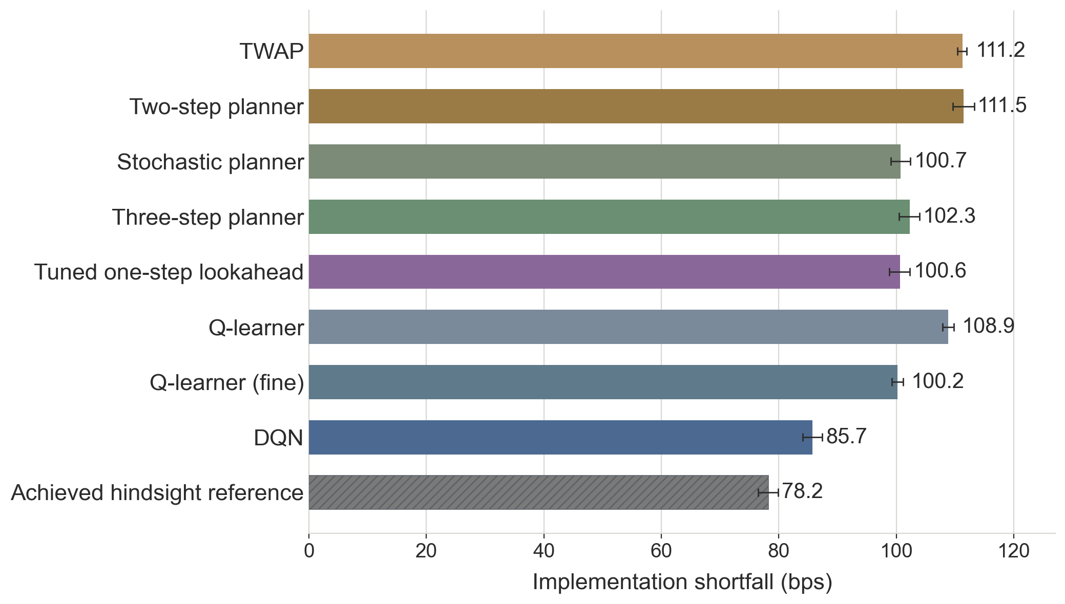
m3_learner_results.csv. The headline result uses a separate reserved block and takes agent-last as its primary ordering.
The DQN advantage may come from timing realized fee and quote variation. The comparison cannot separate that explanation from the limits of shallow search and heuristic continuation.
What better execution looked like
Trajectory diagnostics show three recurring behaviors:
-
Smaller clips. The DQN mostly trades 10% of remaining inventory, averaging about sixteen clips per episode. Tuned lookahead uses fewer, larger clips.
-
Waiting through price run-ups. On representative winning seeds, the policy holds inventory while the oracle rises and executes after the retracement. Lookahead finishes earlier at a higher cost.
-
Trading in lower-fee states. Buy fees fall when a pool sits below the oracle, which is also a cheaper state for the buyer. Pool fees contribute about 33.5 bps of arrival order notional to the DQN’s shortfall. For context, the start-of-step quoted buy fees average about 45 bps across time and pools. These are different summaries: realized fee cash versus the quoted fee state available to the policy.
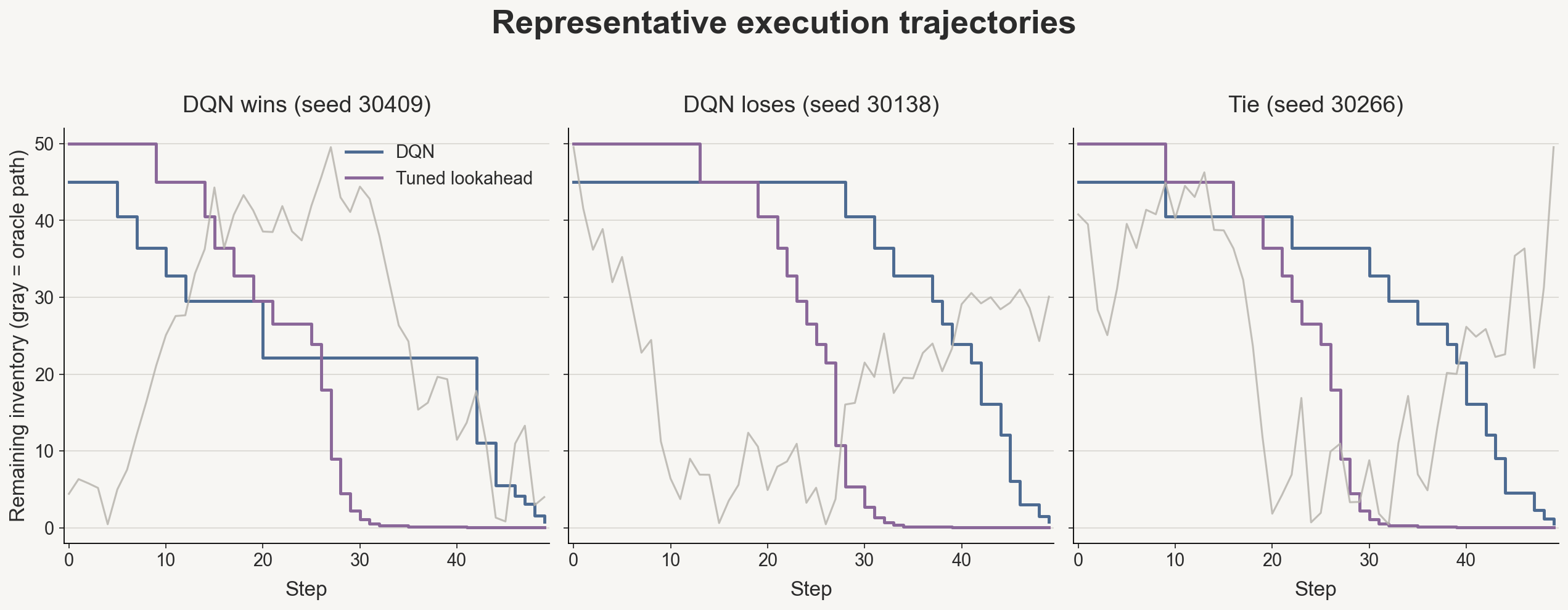
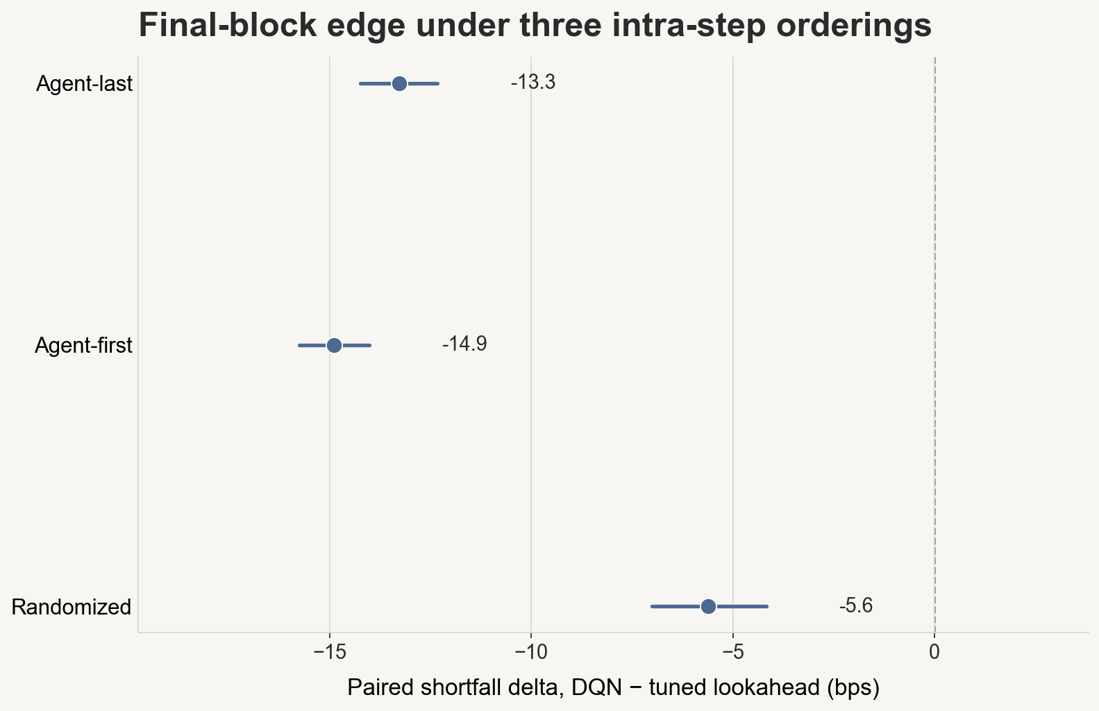
On a final block of 1,000 seeds reserved from model development and first evaluated after the design freeze, with completion forced to 1.0 for every policy, the DQN reduces shortfall relative to tuned one-step lookahead by 13.3 bps under the pre-specified agent-last deterministic ordering and 14.9 bps under agent-first. Fig. 1 is a development diagnostic; these headline gaps come from the reserved final block.
m3r_final_paper_seeds.csv, m3r_reference_final.csv.
Under randomized intra-step ordering, where the controller does not know whether it trades before or after noise and arbitrage, the final-block edge narrows to 5.6 bps. In the 300-seed fee-mode ablation, the paired constant-fee DQN–lookahead estimate is +1.2 bps (means round to 116.1 and 115.0 bps), a near tie (m3r_dynamic_fee_ablation.csv). The larger gains appear in dynamic-fee environments.
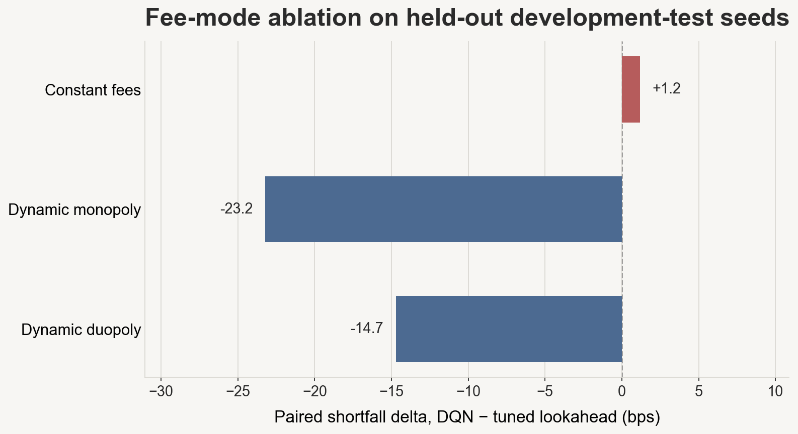
m3r_dynamic_fee_ablation.csv. This is not the final headline block.
The range matters because the measured edge changes with intra-step sequencing.
Closing
Under this closed loop, model-free execution control beats tuned one-step routing, while the shallow planners tested here do not. This is model-conditioned counterfactual evidence. It does not establish live profitability, historical trader behavior, equilibrium of the fee rule, or optimal dynamic fees for LPs.
The tested baseline and weak LP depth-adaptation stresses did not flip the ranking, but richer mempool ordering, block latency, and adaptive LP repositioning remain open.
The simulator (src/sim/), policies, and evaluation pipeline (scripts/rl_equilibrium/) live in egpivo/amm-lab. Frozen paper artifacts are in data/rl_equilibrium/.
Appendix: sources and reproducibility
- Paper: Wang (2026), Reinforcement Learning for Execution under Dynamic Fees in a Closed-Loop DEX Simulator.
- Code and artifacts: egpivo/amm-lab. Simulator:
src/sim/. Pipeline:scripts/rl_equilibrium/. Frozen outputs:data/rl_equilibrium/(m3r_run_manifest.json,final_ladder.csv,m3r_final_paper_seeds.csv). - External references: CoW TWAP documentation; dynamic-fee DEX competition; optimal LP fees; protocol-fee causal study