When Multiple Pools Behave Like One: Impact-Constrained Capacity Concentration in Uniswap v3
An empirical note on effective concentration under a capacity objective.
TL;DR
- 293,273 reconstructed
family × day × direction × impact_bpscells across 78 Ethereum Uniswap v3 token–quote families. - Nominal multiplicity $\neq$ diffuse effective capacity: The cell-weighted median capacity-effective pool count is 1.076 ($N_{\mathrm{eff}}=1/\mathrm{HHI}$), with a median top-1 capacity share of 96.3% and median multi-pool gain $g \approx 3.2\%$.
- Among 36,783 matched family-days, observed pool-volume concentration exceeds reconstructed capacity concentration on 67.6% of days (Spearman $\rho = 0.841$).
- Estimand & scope: Measures impact-constrained capacity at the liquidity layer; gas, routing frictions, MEV, and cross-layer causality are out of scope.
Uniswap v3 exposes several fee-tier pools for the same economic pair. This note asks whether nominal pool multiplicity translates into diffuse impact-constrained execution capacity across sibling pools.
Across 293,273 reconstructed family × day × direction × impact_bps cells in a selected 78-family Ethereum pilot, capacity shares are typically highly concentrated. A family-cluster bootstrap gives a 95% interval of [1.041, 1.128] for median $N_{\mathrm{eff}}$. These intervals quantify sensitivity to the sampled family composition; they do not establish population-level representativeness beyond the selected pilot.
This is a selected multi-pool pilot, not a representative sample of all Uniswap v3 pairs. The broader equilibrium-composition question is motivation only; settlement safety is not estimated here.
What is being measured?
A family is a target token paired with a quote asset (WETH, USDC, or USDT), together with the Uniswap v3 pools in that pair that enter the reconstruction.
For each cell
\[\text{family} \times \text{day} \times \text{direction} \times \text{impact}_{\text{bps}}\]daily pool state is restored from Mint/Burn/Swap history. A capacity optimizer computes (i) maximum notional executable at a fixed impact tolerance on the best single pool, (ii) maximum notional under a split across available pools, and (iii) the capacity shares of that split. Impact tolerances are 10, 25, 50, and 100 bps.
Define the Herfindahl–Hirschman index of capacity shares ${s_p}$:
\[\mathrm{HHI}=\sum_p s_p^2,\qquad N_{\mathrm{eff}}=\frac{1}{\mathrm{HHI}}.\]Under the reconstructed impact-constrained capacity-share vector, $N_{\mathrm{eff}}$ is the number of equally weighted pools that would generate the same HHI. Throughout, I use capacity-effective pool count, capacity-share concentration, or effective pool count under this capacity objective. $N_{\mathrm{eff}}$ is not market power, observed router market share, number of equilibrium competitors, a welfare metric, or a general measure of all execution substitutability.
Let $N_{\mathrm{available}}$ denote the number of pools available to the optimizer in that cell:
\[N_{\mathrm{available}} \neq N_{\mathrm{eff}}.\]The reconstructed capacity allocation is not an estimated Nash equilibrium. It is a fixed-objective optimization. Replay validation on 10,161 swaps (170 pools) has median price error 0.29 bps, with 98.3% under 1 bps—useful for trusting the state engine, not for claiming welfare optimality.
Capacity-gain decomposition
Relative to the best single pool, define capacity gain
\[g=\frac{C_{\mathrm{route}}-C_{\mathrm{best\,pool}}}{C_{\mathrm{best\,pool}}}.\]Among 276,038 cells with finite $g$, 248,449 (90.0%) have $g>0$; median $g\approx 3.2\%$. Because shares are capacity shares,
\[\text{top-1}\approx \frac{1}{1+g}\]holds almost exactly (median absolute gap $8.5\times 10^{-4}$; correlation 0.996). $g$ is useful for describing the incremental capacity contributed by secondary pools, but because the capacity-share construction mechanically links $g$ to top-1 share, it is not treated as an independent concentration result.
Main result: multiple pools, concentrated capacity
The headline statistics below are cell-weighted over family × day × direction × impact_bps cells. A typical cell is not necessarily a typical family.
Across 293,273 reconstructed cells:
| Statistic | Value |
|---|---|
| Median HHI (cell-weighted) | 0.930 |
| Median capacity-effective pool count $N_{\mathrm{eff}}$ (cell-weighted) | 1.076 |
| Median top-1 capacity share | 0.963 |
| Share with HHI $\ge 0.90$ | 56.1% |
| Share with HHI $\ge 0.75$ | 69.2% |
| Share with $N_{\mathrm{eff}}\ge 2$ | 0.67% |
The median cell behaves close to a single capacity-effective venue under the specified impact-constrained objective. Concentration in a dominant fee tier may be economically intuitive; the contribution here is to quantify how much effective capacity sibling pools add at explicit 10–100 bps impact boundaries, rather than infer substitutability from nominal pool count.
Stratifying by available pools:
| Available pools | Cells | Families | Median $N_{\mathrm{eff}}$ | Median top-1 |
|---|---|---|---|---|
| 2 | 266,025 | 68 | 1.083 | 0.960 |
| 3 | 21,984 | 7 | 1.018 | 0.991 |
| 4 | 3,520 | 2 | 1.022 | 0.989 |
| 5 | 1,744 | 1 | 2.082 | 0.602 |
Cell counts are large because families repeat across days, directions, and impact thresholds; the 3- and 4-pool strata contain only 7 and 2 unique families. The 5-pool row is one family only (0x95ad61b0_WETH) and is not generalized. Within this pilot, the 2–4 pool strata do not show greater median capacity diffusion as nominal pool count rises, but cross-family coverage is thin in the 3- and 4-pool groups.
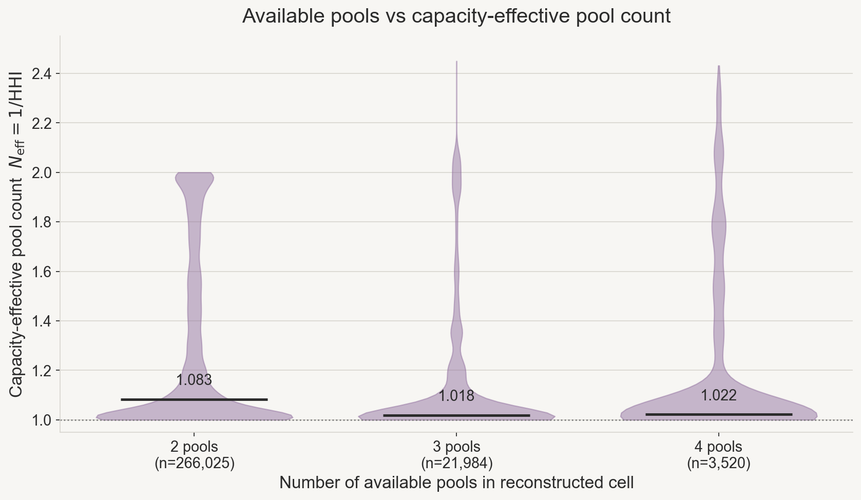
This is descriptive stratification, not a treatment effect of adding a third pool.
How the sample is constructed
The analysis uses a curated multi-pool pilot of Ethereum Uniswap v3 token–quote families. The final manifest (pilot_families.json) lists 79 families and 187 pools. It was drawn from the project’s Ethereum Uniswap v3 event-lake study as a research-curated multi-pool set—not sampled uniformly from all Uniswap v3 pairs. Selection into the manifest required sibling pools that satisfy the inclusion properties below; it may therefore overrepresent families with sufficient event coverage and reconstructible state relative to a random pair draw.
Documented inclusion properties verified from the manifest and pool metadata:
- at least two pools per family;
- at least two distinct fee tiers per family;
- quote assets restricted to WETH (69 configured / 68 in analysis), USDC (6), USDT (4);
- quote-side consistency (Rule A): within each family, the quote asset maps to the same pool side in
quote_map.
78 families produce reconstructible capacity rows. One configured family (0x72e4f9f8_WETH) is excluded because the verified route-capacity run emitted no cells for it. Selection into the manifest did not require successful reconstruction ex ante; that exclusion is an output filter.
Calendar coverage: 2024-01-01 to 2026-06-29 UTC. This is a selected multi-pool pilot and is not claimed to represent all Uniswap v3 pairs. Stage counts and stratum flags are summarized below.
Does the result survive different summaries?
Cell-weighted versus family-weighted
Family-weighted summaries take one within-family median of each statistic, then the median across the 78 analysis families. The aggregate conclusion is not an artifact of families with more days or cells receiving more weight. Family-weighted figures are still summaries of this selected pilot; they are not population-representative.
| Summary | Cell-weighted | Family-weighted |
|---|---|---|
| Median HHI | 0.930 | 0.928 |
| Median $N_{\mathrm{eff}}$ | 1.076 | 1.078 |
| Median top-1 | 0.963 | 0.963 |
Impact tolerance
| Impact (bps) | Cells | Median HHI | Median $N_{\mathrm{eff}}$ | p25 / p75 $N_{\mathrm{eff}}$ | Median top-1 |
|---|---|---|---|---|---|
| 10 | 72,810 | 0.936 | 1.068 | 1.006 / 1.476 | 0.967 |
| 25 | 73,374 | 0.931 | 1.074 | 1.007 / 1.495 | 0.964 |
| 50 | 73,535 | 0.928 | 1.078 | 1.008 / 1.500 | 0.963 |
| 100 | 73,554 | 0.926 | 1.080 | 1.008 / 1.501 | 0.962 |
The result is stable across the impact thresholds tested within the same capacity objective. This does not test sensitivity to gas, fees, latency, or welfare objectives. Medians stay near 1.07–1.08; p25 $N_{\mathrm{eff}}\approx 1.01$.
Family-cluster bootstrap
The 293,273 cells are not independent. Uncertainty uses a family-cluster bootstrap: resample the 78 families with replacement; when a family is selected, include all of its cells. 5,000 draws with fixed seeds; percentile 95% intervals.
| Statistic | Point | 95% CI |
|---|---|---|
| Median HHI | 0.930 | [0.887, 0.960] |
| Median $N_{\mathrm{eff}}$ | 1.076 | [1.041, 1.128] |
| Median top-1 | 0.963 | [0.940, 0.979] |
| Median $g$ (finite-$g$ cells) | 3.18% | [1.89%, 5.25%] |
These intervals quantify sensitivity to the sampled family composition. They do not establish population-level representativeness beyond the selected pilot. The 78 families were not drawn as a probability sample from all Uniswap v3 families.
Quote asset and activity weighting
| Slice | Families | Median HHI | Median $N_{\mathrm{eff}}$ |
|---|---|---|---|
| WETH quote | 68 | 0.931 | 1.074 |
| USDC quote | 6 | 0.943 | 1.060 |
| USDT quote | 4 | 0.870 | 1.149 |
| Top-20 families by matched volume | — | 0.938 | 1.066 |
| Remaining families | — | 0.927 | 1.079 |
WETH-quoted families dominate the cell count, but top-volume and long-tail slices show the same qualitative pattern.
What happens in realized activity?
Reconstruction answers what capacity can look like under the fixed objective. Realized swaps answer a different question: how concentrated is observed family-day volume?
Quote-side human-normalized volume from the pilot daily panel yields family-day HHI over pools in the same family definition. Zero-volume eligible pools enter as zero share. This is pool-log volume concentration, not aggregator routing share.
Matching on family and day gives 36,783 family-days. Reconstructed capacity HHI is averaged over direction and impact tolerance at family $\times$ day.
| Object | Median HHI | Median $N_{\mathrm{eff}}$ |
|---|---|---|
| Observed flow ($HHI^{\mathrm{obs}}$) | 0.955 | 1.047 |
| Reconstructed capacity ($HHI^{\mathrm{cap}}$) | 0.926 | 1.081 |
Pearson correlation 0.741; Spearman 0.841 (bootstrap 95% CI [0.803, 0.869]). Observed activity is more concentrated than reconstructed impact-constrained capacity on 67.6% of matched family-days (bootstrap 95% CI [61.3%, 73.8%]), although the two measures reflect different allocation processes. The median difference is modest, while the strong rank correlation indicates that family-days with high reconstructed capacity concentration also tend to exhibit high realized pool-volume concentration.
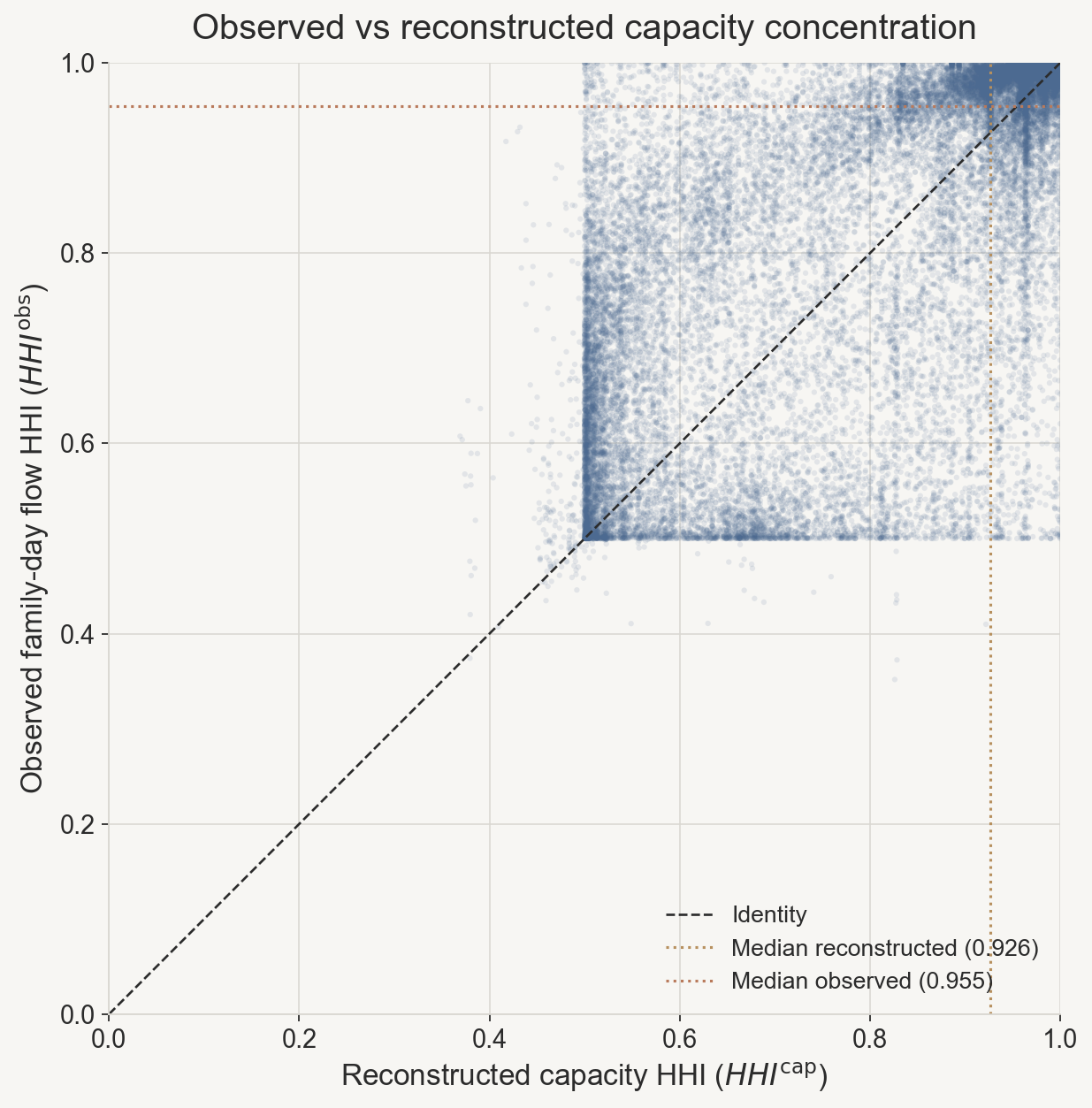
Observed HHI and reconstructed capacity HHI are different objects. The comparison does not imply that traders fail to use capacity, that observed routing is inefficient, or that the optimizer is efficient.
What this does — and does not — show
What this note measures. In a selected pilot, multiple nominal Uniswap v3 pools often map to highly concentrated capacity shares under an impact-constrained capacity objective. Observed family-day volume is also highly concentrated and ranks similarly, although it reflects a different allocation process.
What it does not measure. Gas, fee-aware routing, latency, MEV, failure risk, or Nash play. The optimizer is not a welfare benchmark, and no cross-layer causal claim is made.
Why pool count may mislead. Venue count can be a weak proxy for effective substitutability when capacity remains concentrated under a stated execution objective.
Next observable. When does low $N_{\mathrm{eff}}$ materially reduce execution substitutability for real trade sizes and routes—and at what threshold does ordering-layer concentration begin to affect inclusion resilience?
Reproducibility
Reproducibility package — analysis scripts, processed inputs, manifest, and headline numbers.
Sample construction details
| Stage | Count |
|---|---|
| Configured families | 79 |
| Analysis families | 78 |
| Reconstructed cells | 293,273 |
| Matched family-days | 36,783 |
Excluded: 0x72e4f9f8_WETH (no reconstructible capacity rows in the verified run).
Why this might matter beyond the liquidity layer
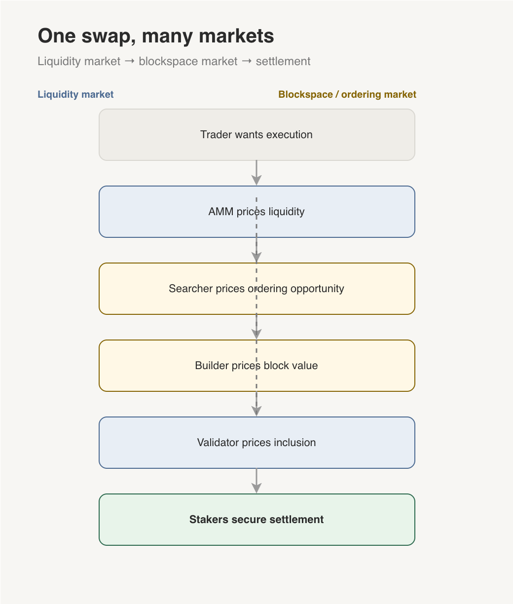
The broader question is whether locally sensible outcomes across three layers
\[G_L=\text{liquidity / execution},\qquad G_O=\text{ordering / blockspace},\qquad G_S=\text{settlement}\]compose into a robust system. Participants optimize layer-local objectives—fees and impact at $G_L$, block value at $G_O$, and protocol constraints at $G_S$—while settlement also depends on properties such as credible inclusion, auditability, censorship resistance, and finality.
The settlement-safe-region framing asks when these local outcomes compose into something like $\mathcal{S}_{\mathrm{safe}}$. That question is motivation only: this pilot estimates impact-constrained capacity concentration inside $G_L$, not cross-layer propagation or settlement safety.
References
- Baggiani, Herdegen, Sanchez-Betancourt. DEX dynamic fee competition. arXiv:2603.09669.
- Heimbach & Wattenhofer. PBS empirics. arXiv:2305.19037.
- Related measurement notes: pool state lab; dynamic fees; same token, multiple markets.