How Far Does a Market Shock Travel?

Two market events, one identification problem, and a block-Hawkes experiment.

The previous piece followed the JPY shock end to end: turnover, risk transfer, exposure, funding path. This one starts from that shock and a second, unrelated market event, and asks a different question — not how big was the move, but how far did it actually reach, and can we ever tell how it got there.

Two shock footprints, SpaceX on-chain wrappers and the JPY cross-market response, next to a block-Hawkes identification test

A shock’s magnitude is easy to measure and, on its own, incomplete. On 30 July 2026, USD/JPY fell about 2.1% in an hour. On 12 June, SpaceX started trading on Nasdaq and at least five tokenized wrappers had to answer for it on-chain. Neither number says how far the disturbance actually reached, or whether anything that moved afterward was actually caused by it.

The first half of this piece measures the footprint of both shocks. The second half asks a harder question the footprint alone can’t answer: when two markets move together, is one exciting the other, or are both just reacting to the same push? That’s an identification problem, and it’s the subject of a controlled experiment — a block-structured Hawkes process, calibrated and tested against a known truth — that this piece reports as its main technical result.

What I mean by a shock’s radius

Call it a shock’s radius, loosely: the set of markets that show an unusually large response, relative to their own normal behavior, in the window after the event. This isn’t a formal estimator; it’s a way of organizing three questions that turn out to be more useful than “how big was the move”:

Localization — which markets moved, which didn’t.
Breadth — did the group of responding markets stay small, or grow.
Persistence — did the response fade, hold, or reverse.

This maps the footprint, not the transmission mechanism. Later, the Hawkes experiment tests why those are different questions.

SpaceX: large local activity, small ending net route flow

At least five tokenized wrappers quote against SpaceX stock — issuer, redemption terms, and route status for each are mapped in Markets Are Full of Roads. SPACEX (PreStocks) is the one under study here: it names SPCXx as its issuer-designated conversion target, with no holder-executable route into any of the other four.

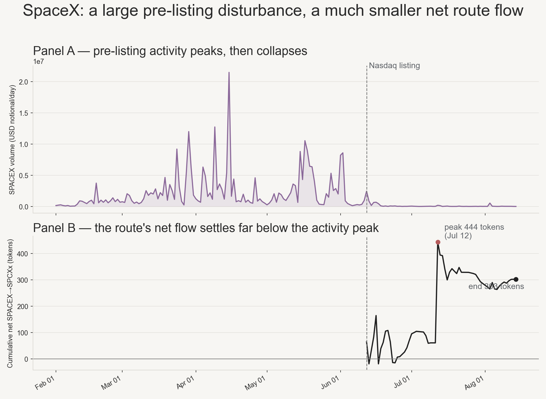
SpaceX activity through time: token volume peaks before listing then collapses; cumulative net route flow peaks in mid-July then declines

Fig. 1. Panel A: daily SPACEX trading volume in USD notional, February–August 2026 (Dune Analytics, Solana). Panel B: cumulative net token flow from SPACEX into SPCXx via their mint-pair swap route. Volume peaks before the Nasdaq listing, not at it, and collapses within weeks of the listing date. The cumulative net flow peaks at 444 tokens on 12 July, then declines to 303 by the end of the frozen window (14 August 2026).

The listing did not coincide with the volume peak. Daily SPACEX volume here is observed raw on-chain DEX volume, measured in USD notional rather than token units; no separate wash-trading classification is imposed on it. Normalized to a 2026-02-12 → 2026-04-30 baseline, SPACEX volume peaked at about \$21.5 million on 15 April, ran at about 0.47× its own baseline during IPO week itself — below baseline — and fell to roughly 0.02× by late June and 0.01× by August. It isn’t listing-specific, either — Markets Are Full of Roads already ruled that out: PreStocks tokens with no IPO to react to fell on the same schedule, leaving the actual cause unidentified.

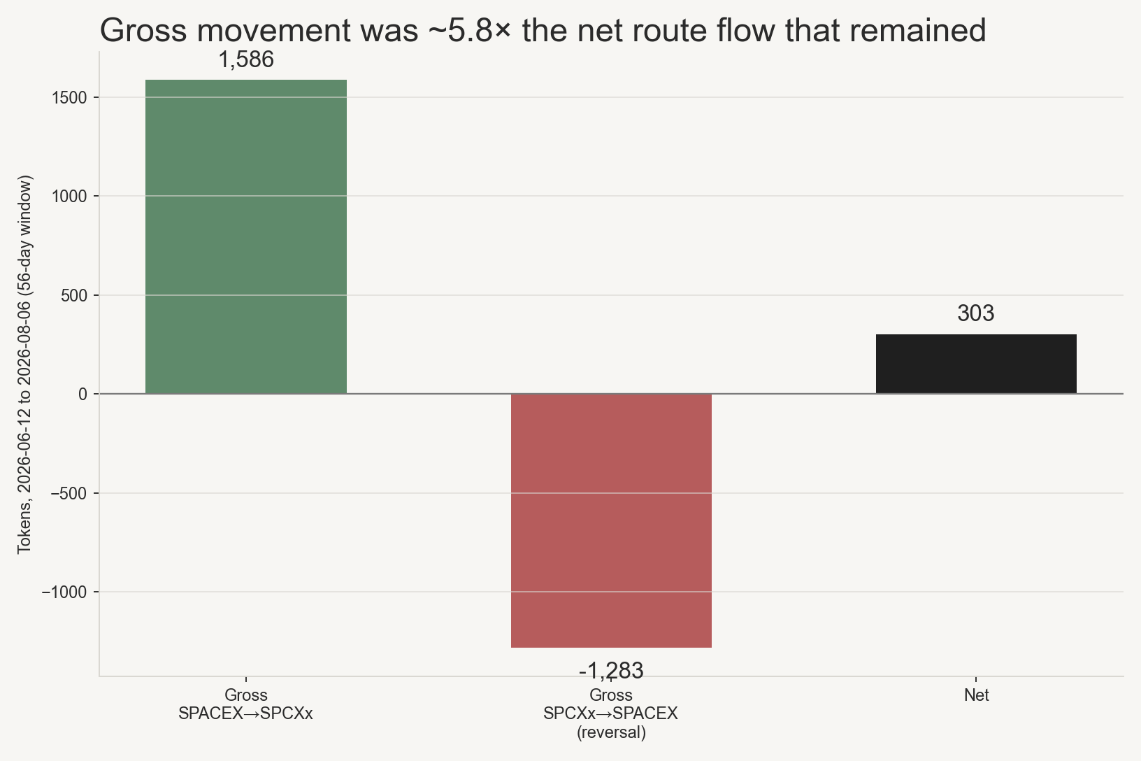
Gross flow SPACEX to SPCXx of 1586 tokens, gross reversal of 1283 tokens, net route flow of 303 tokens

Fig. 2. Full-window (12 June → 14 August 2026, 63 days) mint-pair swap traffic. Gross flow moved 1,586 tokens toward SPCXx; 1,283 moved back; the route's ending net flow is 303 tokens — 19% of gross traffic, 3.5% of SPACEX's 8,742.6-token circulating supply. Same freeze as the 30 August piece. Neither gross nor net identifies one-way holder conversion: the pair also carries ordinary trading and arbitrage, indistinguishable in this data from a one-directional exit.

Large gross movement is not the same thing as a large persistent net flow: most gross traffic is offset in the reverse direction, and the remaining 303-token net balance is an accounting quantity, not a count of holders who converted.

JPY: huge source move, narrow +60m footprint

USD/JPY fell about 2.1% in the hour after 13:35 UTC on 30 July. That clock was frozen from contemporaneous market and wire reporting before the cross-asset analysis was run. Subsequent official reporting confirmed Japanese intervention on 30 July and a coordinated U.S.–Japan intervention on 31 July; those later confirmations validate the intervention episode at the day level, not the specific 13:35 UTC transaction. Against 25 prior same-horizon windows, that native move maps to a robust standardized score, z-MAD, of about −101 — not a literal 101-standard-deviation Gaussian tail, but a genuine signal: USD/JPY’s typical hourly move is small enough (MAD-scaled denominator on the order of two basis points) that even a real ~2% move produces a large standardized number.

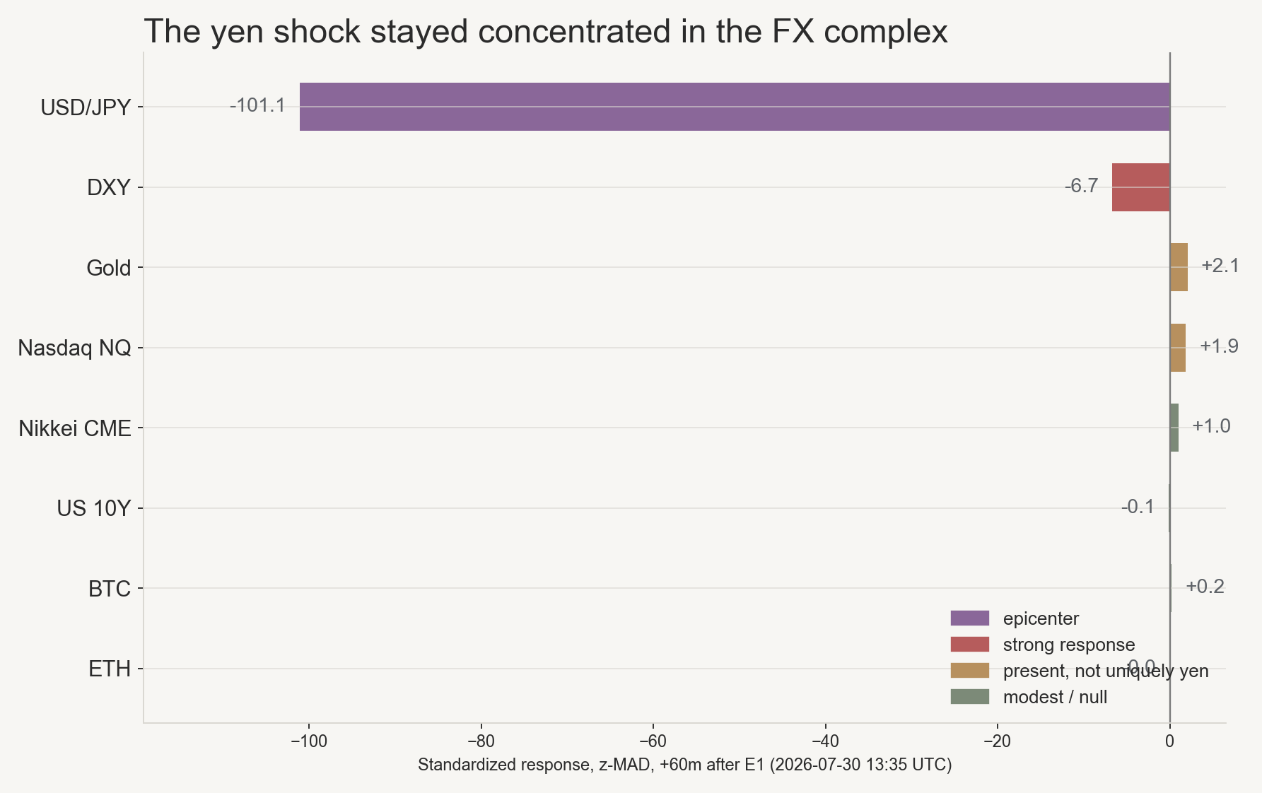
JPY cross-market response: USDJPY and DXY show strong negative z-scores, Gold and Nasdaq show confounded positive responses, Nikkei/rates/BTC/ETH near zero

Fig. 3. Standardized event-window response (z-MAD, against 25 prior same-horizon windows) across eight instruments, +60 minutes after E1. Sources: Dukascopy (USD/JPY), Yahoo Finance (DXY, gold, Nasdaq, Nikkei futures, US 10Y), Binance (BTC, ETH). Gold and Nasdaq moved, but a US GDP/PCE release landed roughly 65 minutes earlier — those two bars are confounded, not transmission evidence. Nikkei (cash closed at E1) shows a modest move; US 10-year, BTC, and ETH are effectively flat.

DXY, the broad dollar index, is the only other instrument that moves clearly: down 0.55%, z-MAD near −6.7 — an order of magnitude smaller than the epicenter, but a legible response in the broader dollar complex. Past DXY, the eight-instrument panel goes quiet: nothing else moves clearly beyond noise once Gold and Nasdaq are set aside as confounded — the previous piece works through that confound, and the Hyperliquid funding-path evidence behind it, in full.

In both cases, the observable response narrows substantially away from the headline quantity. SpaceX’s ending net route flow is a fifth of its gross traffic; JPY’s clean footprint is one currency pair and its closest dollar-complex neighbor.

A footprint is not a propagation path

These charts map the footprint. They do not tell us how the footprint formed.

Two markets moving in the same window are consistent with two different mechanisms. One is common forcing — an outside shock $Z$ hits both $A$ and $B$ independently:

\[Z \to A \qquad Z \to B\]

The other is true propagation — the shock hits $A$, and $A$’s own activity then excites $B$:

\[Z \to A \to B\]

Contemporaneous co-movement, and even simple lead-lag (A moves a few minutes before B), can look nearly identical under either story. A chart overlay can’t tell them apart. The controlled experiment below tests that distinction directly — and it’s why this article doesn’t claim SpaceX’s listing caused anything in JPY, or that JPY caused anything in crypto.

The Hawkes experiment

Separating those two mechanisms needs more structure than a correlation. A Hawkes process models the arrival times of discrete events — trades, fills, price jumps — through a conditional intensity: the rate of new events given everything observed so far. The proof-of-concept fits this directly at the cluster level, not per individual asset: each economic cluster (a currency complex, a wrapper universe, a sector) is represented by one counting process, with K = 5 clusters in total. The fitted model is

\[\lambda_a(t) = \mu_a + s_a(t) + \sum_b \int B_{ab}\, k(t-u)\, dN_b(u)\]

$N_b$ is cluster b’s event process, $\mu_a$ is cluster a’s baseline intensity, $s_a(t)$ is explicit external forcing, $B_{ab}$ is the conditional excitation from cluster b into cluster a, and $k(u)$ is a shared temporal kernel — here the simple exponential $k(u) = \beta e^{-\beta u}$, with $\beta = 1.0$, a characteristic decay timescale of about $1/\beta$. For this proof-of-concept, each economic cluster is represented by one counting process; $B_{ab}$ therefore measures cluster-b-to-cluster-a conditional excitation directly, not a coefficient shared across many individual asset pairs within a cluster. An asset-level block model — many assets per cluster, one shared $B_{ab}$ per cluster pair — is a natural later generalization, but it is not what’s fitted here.

The test object is a single edge: cluster 0 (the source) into cluster 1 (the target), coefficient $B_{10}$. The identification question is a hypothesis test — $H_0: B_{10} = 0$ against $H_1: B_{10} > 0$ — with external shock forcing entered as its own explicit term, kept separate from the excitation term in every world below.

Controlled data-generating processes

The proof-of-concept doesn’t test the model against real data. It tests it against three synthetic worlds where the truth is fixed by construction, so the method can be graded before it ever touches a real market.

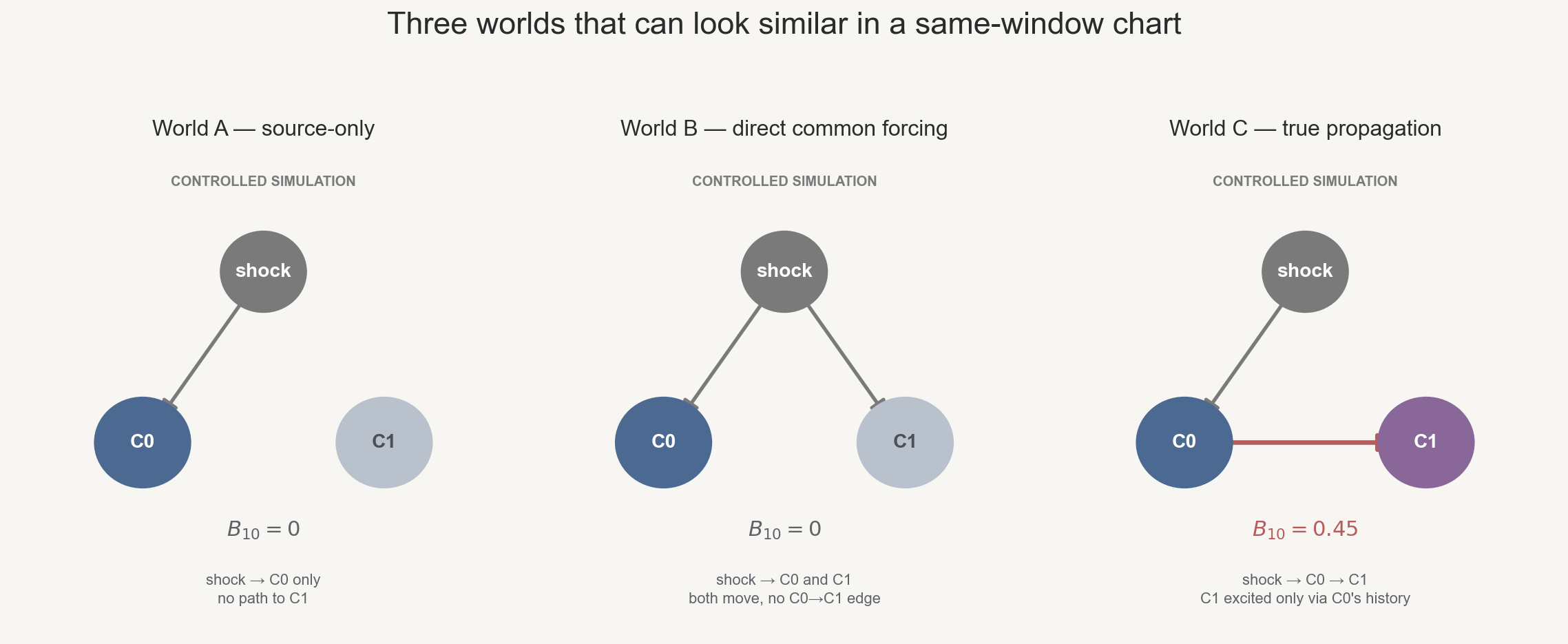
Three controlled worlds: source-only (shock to C0 only, B10=0), direct common forcing (shock to C0 and C1, B10=0), true propagation (shock to C0 to C1, B10=0.45)

Fig. 4. The three controlled data-generating processes behind the calibration and evaluation in Fig. 5. All three are simulations with a known, fixed truth — not empirical claims about SpaceX or JPY. World A: shock hits $C_0$ only, $C_1$ is untouched, $B_{10} = 0$. World B: shock hits $C_0$ and $C_1$ directly, with no edge between them, $B_{10} = 0$ — the hard case, because both clusters move around the same event. World C: shock hits $C_0$ only, and $C_1$ is excited solely through $C_0$'s event history, $B_{10} = 0.45$.

World B and World C can look deceptively similar in a same-window activity chart: both clusters become active around the shock, but only World C contains a $C_0 \to C_1$ excitation edge. World A is the cleaner source-only null: $C_1$ receives neither direct shock forcing nor cross-excitation from $C_0$, so its event process stays at baseline apart from sampling variation. World B is the adversarial case built specifically to fool a naive “both moved, so they must be linked” reading.

Calibration and recovery

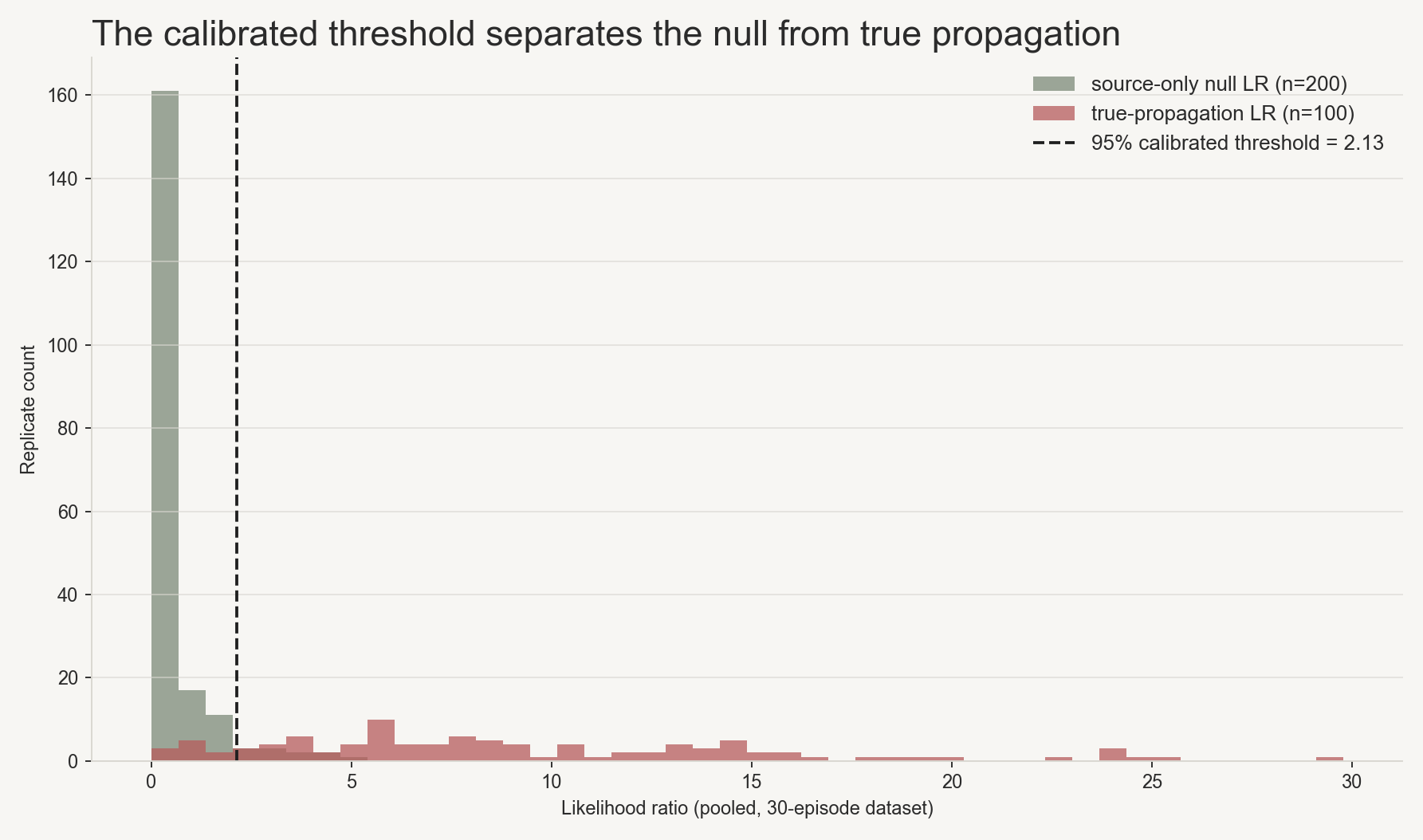
Likelihood ratio distributions: source-only null LR concentrated near zero, true-propagation LR spread out well past the calibrated threshold

Fig. 5. Pooled likelihood-ratio distributions, one shared recovered $B_{10}$ per 30-episode dataset, cluster-level design (K=5, medium regime). The dashed line is the 95th percentile of the source-only null LR distribution itself (200 calibration replicates) — a calibrated threshold, not a generic chi-square cutoff. True-propagation LR (100 evaluation replicates, true $B_{10} = 0.45$) is plotted against the same threshold. Calibration and evaluation replicates are independently simulated — the 200 calibration datasets are not reused in the 100-replicate evaluation runs below.

Under the source-only null (World A), evaluated on 100 held-out replicates independent of the 200 used to calibrate the threshold, the test rejected 4/100 = 4% of the time [Wilson 95% CI: 1.6%–9.8%] — close to the nominal 5% a well-calibrated test should hit. Under direct common forcing (World B), the harder adversarial case, the false-positive rate was 7/100 = 7% [3.4%–13.7%]: both clusters moving around the same shock pushes the test a little further from nominal, but the interval still comfortably overlaps 5%. When a true $C_0 \to C_1$ edge of $B_{10}^{\text{true}} = 0.45$ was actually present (World C), the test detected it 90/100 = 90% of the time [82.6%–94.5%]. Across those same propagation-evaluation replicates, the mean recovered coefficient was $\text{mean}(\hat{B}_{10}) \approx 0.475$ against the true 0.45 — an average upward bias of about 0.025. Per-replicate $\hat{B}_{10}$ values were not archived in the frozen output, so no dispersion statistic beyond that mean is reported here (see the Appendix below).

In this controlled, fully-specified setting, the static block-Hawkes design separates common forcing from genuine cross-cluster excitation with useful power. That’s a statement about the identification strategy, not about any real market: neither SpaceX nor JPY was ever fit with this model, and $\text{mean}(\hat{B}_{10}) \approx 0.475$ describes the simulation, not a claim about how far a real shock travels through real markets.

State-varying excitation remains unresolved

A harder version of the model let the excitation coefficient itself differ between calm and shocked regimes — $B_{\text{normal}}$ vs. $B_{\text{shock}}$ instead of one fixed $B_{10}$. The state-varying extension did not pass its sanity gate. Under the state-null data-generating process (true $(B_{\text{normal}}, B_{\text{shock}}) = (0.45, 0.45)$), it recovered $(0.325, 0.550)$, creating a spurious difference between normal and shock coefficients where none exists. Under the true state-change data-generating process (true $(0.45, 0.80)$), it recovered $(0.275, 0.425)$, preserving the sign of the change but substantially under-recovering its size. I therefore leave the state-dependent extension unresolved rather than debug it further here. Full contour and code are in the Appendix below.

Closing

The two empirical cases show bounded observable footprints: SpaceX’s gross activity was five times its ending net route flow, and JPY’s clean cross-market signature stopped at DXY. Those cases motivate an identification problem but do not identify transmission paths. The controlled experiment is where that problem gets an answer: a cluster-level Hawkes model separates explicit common forcing from genuine cross-cluster excitation with useful discrimination at the frozen design point, while the state-varying extension doesn’t yet pass the same recovery standard.

Markets are connected. Both cases here still had boundaries, and telling why two markets moved together from whether they did takes more than a shared chart window.

Appendix

Hawkes experiment: code and frozen results — gist.github.com/egpivo/911ad78e26a44abc65c9fb86dc6b4aee.
SpaceX: Dune Analytics (dex_solana.trades, tokens_solana.transfers), Helius getAsset. Baseline 2026-02-12 → 2026-04-30; raw on-chain DEX volume in USD notional, no wash-trading filter. Flow frozen 2026-06-12 → 2026-08-14 and activity 2026-02-01 → 2026-08-14 — the same freeze the 30 August piece uses; window medians are true medians. Stamp: shock-to-migration/projects/spacex/data/FREEZE.txt.
JPY: Dukascopy (USD/JPY), Yahoo Finance (DXY, gold, Nasdaq, Nikkei futures, US 10Y), Binance (BTC, ETH).